Inspired by Tamino’s recent efforts at producing a spatially-weighted analysis of temperatures from GHCN stations, I decided to make my own and “Open Source” it. While its currently written in STATA (the statistics software that I use for work), I’d be happy to work with anyone to port it to R or any other language that is a bit more accessible. I hope that folks on both sides of the debate can work together to establish a method of spatial weighting that we can use to do temperature analysis going forward, since it allows us to look at the overall effects of adjustment methods and differing data sets, rather than focusing on individual anecdotes.
The latest version of the source code is available in the Temp_Analysis zip file here: http://drop.io/0yhqyon
The model goes through a number of different steps to generate a grid-weighted global (or local) anomaly:
- Import the data files. Currently the model has been used to import GHCN raw, GHCN adjusted, USHCN raw, USHCNv2 TOB, and USHCNv2 adjusted data, but it should be easily adaptable to any set of temperature data.
- Assign each station to a 5×5 lat/lon grid. This is accomplished by two for-loops that go through each 5-degree increment of latitude or longitude and check to see if each individual station is contained in that increment. If it is, it assigns the midpoint of the range as the station’s lat or lon grid value. Once these loops are complete, it concatenates the lat and lon grid value for each station to a gridbox identifier.
- Weight each grid box by its area. This uses the equation grid_weight = 4 * _pi^2 * 6378.1^2 * cos(lat*_pi/180) * 5/360 * 5/360 sin((latgrid+2.5)*_pi/180) – sin((latgrid-2.5)*_pi/180) to calcuate the relative size of each grid box based on the midpoint (thanks RomanM!). I got this equation from Gavin for interpreting GISS Model E outputs, though he mentioned that it was an approximation and not perfect. If anyone has a suggestion for a better way to calculate 5×5 lat/lon grid box areas, please let me know.
- Optionally apply various filters for different analysis. Filters include restricting stations used by latitude, longitude, country code, U.S. state, urbanity (for GHCN data only right now; don’t have a good urban indicator for USHCN data developed yet), station start year, end year, and duration of station record, as well as custom filters to replicate the Menne analysis and Long document.
- Combine multiple imod records into a single wmo_id record for GHCN data. GHCN has multiple records associated with a single station ID in a number of cases, and this step simply averages all the records available for each station_id. It occurs after the filters are applied, so if you only want to look at rural stations, it won’t combine a rural imod with an urban imod in the rare case that a single wmo_id has both rural and urban records associated with it. In general, the wmo_id / imod differentiation has to do with cases where a station was moved or stopped reporting and was replaced by a nearby station, and mostly applies to locations outside the U.S. This step does nothing at all for USHCN data.
- Calculate the anomalies for each month at each station relative to the 1960-1970 base period, and discard any stations with < 10 years of temp data per GHCN methodology. This also discards all wmo_ids without a record in the 1960-1970 period. This is the part I’d like to improve, since it reduces the stations available by about 15% in GHCN data. Note that this has no real effect on USHCN data, since virtually all stations reporting currently have data from the 1960-1970 period.
- Average the anomaly of all stations in each grid cell for each month to obtain the grid cell anomaly.
- Calculate a grid-weight for each month of each grid cell in each year, where the grid weight is equal to the cell’s grid area divided by the total grid area of all grid cells available for that month.
- Multiply the each grid cell anomaly by the grid weight for each month of each year and sum up the results across all grid cells to obtain the average by month.
- Calculate the annual average anomaly via a weighted average of each monthly anomaly by the number of days per month, taking leap years into account.
We can do some initial validation (to make sure things aren’t too screwy) by comparing GHCN raw data to GISSTemp land temperatures. Note that we don’t expect this to be perfect, because GISS adjusts GHCN data (and actually lowers the global temperature vis-a-vis the raw data, as both this analysis and a similar one by Jeff Id show). The Rural/Urban designation here is based on GHCN station metadata; it may not be perfect, and we can try other collections of stations that we identify as rural or good if we want (indeed, we do this with CRN12 stations in the U.S. later on).

We can also compare stations with records post-1992 to those without, to quickly replicate the work that Tamino and the CCC folks did on addressing E.M. Smith’s whole station dropout arguement:
 Since no one has looked into it yet, we can consider the case of Northern Canada and see if station dropout there has had any effect on temperatures:

Lets take a look at just the U.S. for a bit, since its where a lot of the criticism of temperature data has been centered.
We can start by looking at Raw and Adjusted GHCN data stations in the U.S. Lower 48:

And break these stations down into Rural vs. Urban (using an 11 year running mean to smooth out some of the noise):

In addition to the 400 or so GHCN stations in the U.S., we also have access to 1200+ stations in USHCN. Lets incorporate those into our model, and look at raw GHCN, adjusted GHCN, raw USHCN, adjusted USHCN, and GISS for the lower 48 U.S.:

Since GISS uses adjusted USHCN as an input (and further tweaks it), we should expect those series to be quite close. Indeed, we find:

USHCN and GHCN use somewhat different adjustments for Lower 48 U.S. stations. Lets compare them:

Now, USHCN doesn’t have a simple Urban/Rural designation in the Metadata. I’m working on trying to figure one out from the station landuse data, but for the time being we can use Anthony and the SurfaceStation.org effort as a first pass (essentially replicating the work of Menne et al 2010). Here are all 71 CRN12 stations compared to the CRN345 stations:

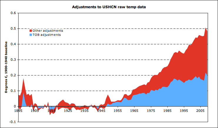
Similar to Menne et al, we find that “good” CRN12 stations have a slightly higher anomaly than the “poor” CRN345 stations using the raw USHCN data. We can also take a look at the adjusted USHCN data. There are two primary adjustments made to USHCN raw data in USHCN v2: time of observation (TOB) adjustments, and urbanization/discontinuity adjustments. Here are CRN12 stations for all three datasets (raw, TOB, and fully adjusted).

The majority of the adjustments that occur are TOB-related, but there are also non-TOB positive adjustments to the “good” stations, which is interesting. Lets compare this to the adjustments made to CRN345 stations:

Here we see that both the TOB adjustments and the additional adjustments are larger for CRN345 stations than for CRN12 stations, which is a good sign. The difference between CRN12 and CRN345 stations in each dataset bears this out:

After each round of adjustments, CRN345 stations become closer to CRN12 stations. However, the net adjustment to both stations are still positive, for both TOB (which is expected) and non-TOB adjustments. Lets looks at the non-TOB adjustments done to CRN12 and CRN345 in more detail:

Anyhow, thats it for now! If you have suggestions to improve the model, or things you are interested in seeing analyzed, let me know. Also, please download the source code (if you run STATA) or work with me to port it over to R (if you don’t) so you can play around with it yourselves.
Also, click on images to embiggen! And thanks Lucia for giving me a chance to do I guest post on my recent work. 🙂
Nice job, I won’t have time to review this in detail until later but from the result, it looks like great work.
A spot of integration tells me that the area of a box bounded by lines of fixed latitude (north and south) and lines of fixed longitude (east and west) is:
R^2 (long2 – long1) (sin lat1 – sin lat2)
where long1, long2, lat1, lat2 are the longitudes and latitudes in question. Sanity check: these are biggest at the equator (where sin lat changes fastest) and zero at the poles (where sin lat doesn’t change). Constant factor check: when the box is the whole sphere, long2 – long1 = 2pi, sin lat1 = 1, sin lat2 = -1, so area is 4 pi R^2. Correct.
R is 6378 km, more-or-less, and if you have 5-degree boxes, then long2-long1 is 5 degrees which is pi/36 radians, so the R^2 (long2-lon1) factor is 3.55e6 km^2. sin lat1 – sin lat2 varies from 0.087 when lat2 is 0 (the boxes adjacent to the equator) to 0.0038 when lat1 is pi/2 (the boxes at the poles).
Here’s a complete list of box areas, depending on latitude, in square km.
0-5: 309394
5-10: 307040
10-15: 302348
15-20: 295356
20-25: 286115
25-30: 274698
30-35: 261189
35-40: 245693
40-45: 228327
45-50: 209223
50-55: 188527
55-60: 166396
60-65: 142999
65-70: 118513
70-75: 93125
75-80: 67029
80-85: 40423
85-90: 13508
I hope this helps.
Zeke – I think your efforts are admirable, though I think to be truly resolve questions with the temperture history a thorough station by station QA/QC of the raw data station data is going to be necessary. Nonetheless, a couple of questions about what you are doing.
One, have you or anyone else for that matter considered establishing a grid of equi-area triangles to use as the gird cells rather than using 5×5 lat-long. In many ways, this might make the problem of area-weighting the grid cells go away as well as make interpoloation/extrapolation of cell values for cells without data a bit easier. However, from a programming persepctive, this would be substantially more difficult and I am not sure how one would go about it.
Two, how do you (if you do it at all), estimate cell values for cells where there is no station data? I didn’t see any explanation for this in your post above.
From the old thread:
TOB adds the most in both cases, but non-TOB adjustments are positive for both. This makes sense for CRN345 (since they are lower than CRN12), but the fact that the magnitude of non-TOB adjustments is almost the same for CRN12 is a tad odd.
Put aside for a moment how CRN12 and CRN345 compare to each other. The cited document says that CRN345 are ranked as such because of artificial heating issues. How do you justify adjusting anomalies UPWARD when you just stated that the station is affected by artificial heating? And again, forget about whether CRN345 is higher or lower than CRN12.
Zeke, The old USHCN .txt file to describe stations has changed from
what it was before. It used to have a ton of metadata.
I’ll look for an old version. What data elements do you have for GHCN?
Nick,
The method I’m currently using gives me almost the same numbers, except in the +/- 85-90 lat range where is significantly underestimates the size.
I also discovered a programming error where it was using the the individual station latitude rather than the station’s grid’s midpoint latitude to calculate grid area. Shouldn’t make much of a difference, but I’ll fix it quick and double check. Hope I don’t have to remake all the figures above 😛 Oh well, that’s the benefit of making everything public, tease out the bugs quickly.
Argg.
Zeke. You can get pop data here:
First:
http://cdiac.ornl.gov/ftp/ushcn_monthly/station_inventory
Then look at the other files for example
http://cdiac.ornl.gov/ftp/ushcn_monthly/station_landuse
All this info used to be in one easy to read file??
torn8o (Comment#35773) March 1st, 2010 at 12:29 pm
CRN345 are ASSUMED to have a bias. Whether they do or not
has yet to be determined.
But lets suppose that CRN345 is BIASED by 1C up.
We start out with a place where the temps dont change.
1,1,1,1,1,1,1,1
Then somebody changes the TOBS..
1,1,1,1,1,1,1,1,.5,.5,.5,.5
Then we continue to collect data and we get the following
1,1,1,1,1,1,1,1,.5,.5,.5,.5, 1,1,1,1,1
Then Somebody looks at the data and says hey? There was a TOBS change! So the team adjusts the series by .5 and you get this
1,1,1,1,1,1,1,1,1,1,1,1, 1.5,1.5,1.5,1.5,1.5
Got it?
Then somebody looks at the site and says hey! that site is a CRN5
here are the questions
1. Does the series go to 1.5 because of CRN5?
2. When it become CRN5?
3. Is CRN5 the only explanation or is it really warming
CRN5 and TOBS are two DIFFERENT adjustments. TOBS has been modelled. That science can be checked.
With CRN ratings you dont have any MODEL of the effect.
You have a “scale” that says CRN5 is bad. how bad? well
you have to measure.
ALSO, with CRN rating you have the inherent problem that you dont know WHEN the site went bad, so you cant adjust, you can only drop it.
Jeff,
I think one of the issues that is going to come up fast on people is the metadata. I started looking back at the old ushcn stuff and the files have changed. The used to have flags for rural, airport, equipment type, land use, nightlights, brightness index, ground cover..
Thanks Mosh, I’ll try and work out a station classification from those when I have time.
.
Thinking about it a bit more, I kinda like the method I accidentally created by using individual station latitude in generating the grid weight. Essentially, what its doing is giving each station a weight equal to the area of a 5×5 lat/lon grid with that station at the center, and giving the overall standard 5×5 grid box containing the station(s) a weight equal to the average of a 5×5 grid box around each station. So a grid box that has most of the stations at a lower latitude (e.g. closer to 0 latitude) has a slightly higher weight than a grid box at the same standard latitude with most of the stations at a higher latitude within the grid box, which actually is desirable. That said, it appears to have very little effect:
http://i81.photobucket.com/albums/j237/hausfath/Picture121.png
http://i81.photobucket.com/albums/j237/hausfath/Picture120.png
.
I’ll double check the Menne analysis as well.
BobN,
Nope, but if you can figure out the equations to do triangles I’d be happy to give it a whirl. As far as what happens when a grid box has no data, the weights of all the other grid boxes increase proportionately, since the grid weights are calculated for each individual month for each station relative to the total grid area covered by all the data for that month. This means that if too many grids drop out you might start seeing regional factors crop up, but there is no easy way of avoiding that.
Zeke:
Thank you. This is a very impressive piece of work and will force us all into more fact-based and substantive discussions, however distasteful that might be.
In the 5th graph (Picture-1101.png) and the 8th (Picture-114.png) almost all of the adjusted temps are lower than raw prior to 1965 and higher afterward. Why is that?
Would it be wrong to say that based on available data as you see it that UHI and site bias contributes at least 0.05 deg C but not more than 0.15 deg C of warming?
Thanks again. Well done.
Zeke,
Also check with Ron. He did a very differenet approach for rural/urban and used circa 2000 gridded GIS data ( down to 2.5 arc minutes)
Stop by his site and see if he can see fit to post a file with
Station names and identifiers and the pop figures.
If not, somebody else can go to the same source ( columbia sedac) and pull the numbers.
I guess my analytic approach would be this:
Develop a screen to remove all possible contaminting
influences.
A. Select stations that are not at airports
B. Select stations that are away from sea coasts ( lower warming trends possible )
C. Select stations that have Dark pixels on the OLS nighlights
data.
D. Select un populated areas ( see the gridded pop data)
E. In the US select CRN12
That gives you a good shot at finding rural stations that are well sited
Zeke,
Good stuff. No doubt.
In all of this, is there a way of demonstrably separating out the “A” factor in the data?
George,
All the graphs that show series with diverging trends (e.g. one series having higher trend than the other) will tend to show some of that divergence before the 1960-1970 baseline and some after. The reason for this is because each series is baselined relative to its own 1960-1970 values, not the values of the other series that it is graphed with. I could redo the graphs by picking a reference series and rebaselining all the other series to that reference, but it wouldn’t matter all that much.
Re: Steven Mosher:
Ok – I got it. I thought the non-TOBS adjustments were trying to adjust for the artificial heating in CRN345. I understand now that there is no adjustment. They are just stating that the station’s data might be questionable.
A couple of things that stand out to me though:
The non-TOBS are almost always down prior to 1972 and almost always up after.
Speaking of TOBS, in Fig. 4 of Quayle et. al, 1991, if you take month 0 to be approximately 1987, the average temperature trended down from about 1980 to about 1990 for the more than 1000 stations they used in that study. That is opposite of what you see in Zeke’s plots.
The CRN12 minus CRN345 adjusted shows CRN12 stations warming more than CRN345 in the more recent years. I would have expected to see it the other way.
I’ll do some more digging on the “other” adjustments.
here Zeke
http://www.surfacestations.org/USHCN_stationlist.htm
best I can do for now
Some of the feilds are run together. I can decifer if you like.
Nice work Zeke.
I’ll build a file of station ids, lat, lon, alt, population density tonight. That way anyone can pull it down for use as a filter.
Of course, with the speed you’re going these days, you’ll probably have it done before I finish typing this message. 🙂
Mosh,
Thanks. I’ll play around with it after work.
.
torn8o,
You need to remember that “down” is relative to the baseline, which is calculated relative to the values of each series. This means that the difference charts are a tad misleading in their magnitude, though their trends are correct. I’ll see what I can do to fix that… It explains why you see the “0” mark around 1960-1970 for all of the series.
torn8o,
Everything is zeroed at 1960-1970 because that is the baseline for each series. I’ll try and figure out a way to plot multiple versions of the same temp on a fixed baseline instead of a series-specific one for better comparisons, but the trends shown are baseline-independent.
Zeke:
I think 10 years may be too short a baseline for the station combining method you are using. I’ve not studied this quantitatively, but it’s something to examine before getting too far.
Clearly, one or two years is too short a baseline; how long is long enough? This could be tested; as you increase the baseline length the ‘answers’ in any given grid box should converge on some stable results, until you start losing stations and you end up undersampled.
But all this can be avoided. You can do as you wish, but in my opinion, the first difference method is the best way forward. Apologies to Tamino.
Actually, if you were somewhat ambitious, you could give the user the choice of station combination methods.
carrot eater (or Chad),
Any handy reference to the equations used by the first difference method?
Nice work Zeke. I do appreciate your time and efforts reworking these temp records.
Can we draw any sound conclusions from this? An in-depth analysis of the temp record is probably above my pay grade. Here is what I see: Some UHI effect over the last 20 years in the raw data, some adjusted temps that appear to exaggerate warming trends as much as .15C. In spite of these findings there is clear and present warming over the last 100 years. Anything I missed? Your conclusions?
Another thought: you are losing information by only looking at Tmean. Interesting things can come of looking at Tmax and Tmin separately, as they show different behaviors.
Nobody should be assuming that CRN 345 have any predictable and systematic bias at all, without looking at the data. Menne 2010 suggested that CRN 345s tended to be stations that switched to MMTS, while CRN 12s tended to be the old LiGs, but this isn’t a hard rule. Menne 2009 had previously suggested that a priori, one cannot know the required adjustment for a switch to MMTS – it could be warming, it could be cooling, it could be nothing, it could have any of a distribution of magnitudes. This is a definite revision of the findings in Quayle 1991. Simplistic statements on the basis of CRN ratings are to be avoided.
Menne mentioned that a sensor change introduced bias which would justify some of the adjustments – if the adjustment is single step change.
The TOBS adjustments are suspicious because they should be step changes – not ramps because the time of observation does not change gradually over years. Also changes to DST would affect this bias in some months.
I also question whether the real bias is as large as claimed since the bias is only introduced when a cool day follows a warm day and the time of observation occurs near the maximum for each day.
It is possible that this bias is being over corrected for many stations but we can’t know because it is not possible to calculate the true magnitude of the bias without real data.
Zeke,
I think it’s pretty straightforward in concept. See Peterson et al, “First difference method: Maximizing station density for the calculation of long-term global temperature change” GRL 103: 25,967-25,974 (1998).
At the simplest implementation, your equations are: Subtract year-on-year monthly values. Find the average of this difference. Then add it all back together again to reconstruct a temperature history. Then recenter the series on whatever baseline you want.
No adjustments for elevation needed?
If an individual station changed elevation due to a station move, you’d make an adjustment to that station at the time of the move. But none of the bloggers are doing any such adjustments yet (that’s the much harder part); just the raw data.
The TOBS adjustments are suspicious because they should be step changes – not ramps because the time of observation does not change gradually over years.
.
actually it does.
more and more stations changing to a different time will give you a ramp.
.
It is possible that this bias is being over corrected for many stations but we can’t know because it is not possible to calculate the true magnitude of the bias without real data.
.
there is plenty of daily weather data on the web. you can test it as much as you like.
Carrot Eater,
At least for the U.S., the 1960-1970 baseline doesn’t matter too much. I ran the model with a 1940-1980 baseline instead (which is fine for USHCN, since just about all the records have durations that cover that period; it would run into some secondary effects with GHCN global temps because it would cause a lot more stations to be excluded from the analysis). The maximum difference between the 1960-1970 and 1940-1980 baseline runs was only around 0.005 C.
Ah, good news, Zeke. Good to do the due diligence; people would question you using an anomaly method on a shorter baseline than others, so it’s good to be prepared to defend your choice.
I still prefer the First Difference method, since I think it handles certain discontinuities better. But on the global scale, it doesn’t much matter.
Carrot,
I agree that it would be a better approach, I just need to figure out how to code it (or convince someone to take the initiative and do it themselves).
.
For folks asking about TOB vs. other adjustments to USHCN, here is a graph that might be a tad clearer:
http://i81.photobucket.com/albums/j237/hausfath/Picture123.png
sod,
Analyzing hourly data only tells you what the bias is for the location where the data was collected during the time it was collected. It does not tell you what the bias would be if you only have min/max data for different station at a different time with a different instrument.
Carrot Eater:
First difference also results in a noise amplification of sqrt(2). For it to be the better method, the improvement in bias error it offers needs to offset this.
Zeke,
Very nice work…. with no bile and no arrogance. Perhaps you can be a leader of the next generation of climate scientists. 😉
.
Now, if we could only actually read the details and rational for the various adjustment procedures, we could start to see if the (large) adjustments to the raw data make any sense.
Now, if we could only actually read the details and rational for the various adjustment procedures, we could start to see if the (large) adjustments to the raw data make any sense.
See if any of these help:
Easterling, D.R., and T.C. Peterson, 1995: A new method of detecting undocumented discontinuities in climatological time series, Int. J. of Climatol., 15, 369-377.
Karl, T.R., C.N. Williams, Jr., P.J. Young, and W.M. Wendland, 1986: A model to estimate the time of observation bias associated with monthly mean maximum, minimum, and mean temperature for the United States, J. Climate Appl. Meteor., 25, 145-160.
Karl, T.R., and C.W. Williams, Jr., 1987: An approach to adjusting climatological time series for discontinuous inhomogeneities, J. Climate Appl. Meteor., 26, 1744-1763.
Karl, T.R., H.F. Diaz, and G. Kukla, 1988: Urbanization: its detection and effect in the United States climate record, J. Climate, 1, 1099-1123.
Karl, T.R., C.N. Williams, Jr., F.T. Quinlan, and T.A. Boden, 1990: United States Historical Climatology Network (HCN) Serial Temperature and Precipitation Data, Environmental Science Division, Publication No. 3404, Carbon Dioxide Information and Analysis Center, Oak Ridge National Laboratory, Oak Ridge, TN, 389 pp.
Menne, M. J., C. N. Williams, and M. A. Palecki (2010): On the reliability of the U.S. Surface Temperature Record, J. Geophys. Res., doi:10.1029/2009JD013094, in press. (accepted 7 January 2010)
Peterson, T.C., and D.R. Easterling, 1994: Creation of homogeneous composite climatological reference series, Int. J. Climatol., 14, 671-680.
Quayle, R.G., D.R. Easterling, T.R. Karl, and P.Y. Hughes, 1991: Effects of recent thermometer changes in the cooperative station network, Bull. Am. Meteorol. Soc., 72, 1718-1724.
You can get links to most of these over here:
http://rhinohide.wordpress.com/ghcn/
Hooray for real science!
Genuine replication!
Zeke Hausfather (Comment#35783)
March 1st, 2010 at 1:25 pm
…but if you can figure out the equations to do triangles I’d be happy to give it a whirl.
or, as Steve McIntyre put it so much better a couple of years ago:
Gridding from CRN1-2
Gridding is a type of spatial smoothing for which there are a variety of standard functions and no need for people to ponder over triangles or hexagons (which don’t matter much) or to write new code.
In order to assess the 2006 anomaly in John V’s 2006 calculation reported previously, I’ve calculated a gridded anomaly for the U.S. using standard spatial smoothing software in R. This enables the calculation to be done in a few lines as explained below. I’ll also show results which reconcile most of the results to date. I’ve shown the details of calculation step so that there will be no confusion. I also want to show how simple it is to produce gridded data from station data. It only takes a couple of lines of code. http://climateaudit.org/2007/10/04/gridding-from-crn1-2/
Those of you who have belittled SteveMcIntyre and his work should in fact be gobsmacked at his volume of output, and its’ elegance and accuracy.
Zeke,
One thing that isn’t clear is which of the data series are computed by you, and which are somebody else’s published record. I’m guessing you computed all of them, except the ones labeled as ‘GISS’?
The NCDC also does gridding for itself; you could also append their results to see how closely you match them.
Ron: You need Menne and Williams 2009 on there. “Homogenization of Temperature Series via Pairwise Comparisons” Journal of Climate 22: 1700-1717 and Menne/Williams/Vose, “THE U.S. HISTORICAL CLIMATOLOGY
NETWORK MONTHLY TEMPERATURE
DATA, VERSION 2”, in BAMS (2009). These two papers describe USHCN v2.0, and supersede everything previously written about USHCN except for the TOB papers.
Carrot,
You are correct that GISS (for both the globe and lower 48) is the only series I currently compare to. I’ve downloaded NCDC monthly temps for the globe, and I’ll compare them with my monthly GHCN v2.mean_adj outputs. However, I’m not sure where to find NCDC temps for the lower 48 by month or year; any suggestions?
Can’t be science, where are the accusations of fraud and incompetence?
Nice work Zeke,
I guess the big question we all have is why is the trend upjusted upward by over 0.5C since about 1915. This is actually higher than the total increase in temperatures in the US lower 48. [I know, a half-dozen papers explain the mechanisms but these are still semi-self-serving for those desiring to increase the record to match the theory].
Then, the next question is what is the adjustment made to the global temperature record. The answer is we don’t actually know that but it is probably a little higher than the US lower 48 which is supposed to be best network in the world and has more transparency than the global record.
In terms of weighting for the global temperature record (not as relevant for the lower US 48), some adjustment must be made for the relative size of the Earth at different latitude bands. 70N to 80N is only 2.3% of the total Earth surface area while 0 to 10N is 8.7%.
Bill,
All processed temperature series (GISS, HadCRUT, NCDC) seem to report lower temperature records for the global land areas than we see from the GHCN raw data. Its mainly in the U.S. that adjusted temps are considerably higher than raw temps.
The weighting algorithm used takes into account the size of the Earth at different latitude bands; see Nick Barnes’ post earlier in the thread.
Ron Broberg (Comment#35830),
Thanks, only a couple left behind a pay wall.
Lol, so Lucia basically did in a few days a more thorough analysis than Tamino did in his “month.”
True, except it was actually a very fine job by Zeke
Michael–
I didn’t do the analysis. Zeke did. I’m not sure, but the first to do an analysis may have been Zeke. The first with area averaging may have been Roy Spencer. Then Tamino, then Nick Barnes.
But… I’m not sure. No matter what, Ididn’t do anything.
“I got this equation from Gavin for interpreting GISS Model E outputs, though he mentioned that it was an approximation and not perfect. ”
Ach. Near enough for ‘climate science’.
As a lurker, I applaud the quality of Zeke’s work and the focus on technical issues on these threads. Properly analyzed and presented data are worth more than arguments.
Lucia,
“No matter what, I didn’t do anything.”
.
Not true, you host a place where it is possible to have meaningful technical exchange, which really is something.
bugs (Comment#35842),
“Can’t be science, where are the accusations of fraud and incompetence?”
This might be a good time to lighten up a bit. Zeke has done some good work, posted his code, kicked around some ideas, and invited comments/suggestions. People have mostly applauded his efforts, and I do as well. So what exactly is there to complain about?
Recommend checking Radius R = 6378.1.
This appears to be the Equatorial radius in km.
However NASA’s Earth Fact Sheet lists:
I would guess that a first order surface approximation should better use the volumetric mean radius of 6371.0 km rather than the equatorial radius.
The next refinement would be to use an equation that accounts for the oblate distortion of the surface due to the earth’s rotation. Any specialists who could track that down?
Michael,
I wouldn’t go that far; Tamino did a much more interesting method of combining station records than I did. That’s one part of this model that I definitely need to improve. One of the reasons I’m focusing mostly on U.S. temp analysis at the moment is that I don’t trust my global calcs quite as much yet for precision analysis, though they probably aren’t too bad.
carrot eater (Comment#35803) March 1st, 2010 at 2:39 pm
“Another thought: you are losing information by only looking at Tmean. Interesting things can come of looking at Tmax and Tmin separately, as they show different behaviors.”
AGREED. Tmax is going to be hit in the following ways.
1. Increase. BUT ONLY if there is a radiative canyon. I dont
see any sites with radiative canyons ( like a corner reflector
that would focus IR energy or trap it )
2. Decrease if there is shading.
Tmin is the most likely variable to be hit. Changes in physical geometry are going to change the boundary layer and the turbulent mixing. Tmin can also be hit by the delayed release of
heat from heak sinks like concrete.
“Nobody should be assuming that CRN 345 have any predictable and systematic bias at all, without looking at the data. Menne 2010 suggested that CRN 345s tended to be stations that switched to MMTS, :
Agreed the bias can go in both directions, Heat sinks and physical
structures which change the boundary layers.. case by case basis
“while CRN 12s tended to be the old LiGs, but this isn’t a hard rule. Menne 2009 had previously suggested that a priori, one cannot know the required adjustment for a switch to MMTS – it could be warming, it could be cooling, it could be nothing, it could have any of a distribution of magnitudes. This is a definite revision of the findings in Quayle 1991. Simplistic statements on the basis of CRN ratings are to be avoided.”
Quayle’s report ( from memory) was just a side by side assessment. Two well sited sensors. in situ all bets are off.
Lucia, you did something…you let Zeke post here, and then you didn’t take credit for work you didn’t do! 😉
Zeke, I like your breakdowns of specific areas and situations far more than Tamino’s.
Obviously I need some ZZZZ’s, because my accuracy and productivity today are horrific!!!
. Ron,
The other cool thing to have would be a nightlights data set for all the lat lons..
NVGI ( vegatative index would be cool as well)
Carrot Eater:
I meant to say I thought this was a really great idea, btw.
Tmin is expected to be more strongly affected than Tmax. It would interesting to see if this gets reflected in the data.
Have I understood correctly that the GHCN USHCN “raw” data being used is monthly? As folks do not sample temp monthly, it is not raw in the sense of being what was read directly. Would it be possible to use daily, ie is it available for much of the period, and across the world?
sean
Daily is available for some places.
Lucia,
can you please give ron a link in the blog roll? TIA
Carrick
It might be interesting to see how FDM works instead of applying a TOBS adjustment. Since the TOBS adjustment is a discrete jump only a small number of time during a whole series, it seems it would make more sense to drop the month the OBS time changes and use FDM.. make any sense?
So
Steven M, will you be explaining to Mr Watts that the conclusions he reached with Joe D’Aleo in their diatribe were wrong? He doesn’t seem to want to admit it.
Sean,
Yes, GHCN is called raw, but somebody had to average some numbers together. Roy Spencer used a database that’s a step more raw than that, but most everybody has no experience using it yet (and it will eat up your hard drive).
David Hagen:
The earth isn’t a perfect sphere, but how much does it really matter? There’ll be a little error in the calculated relative areas; so what.
Zeke:
“All processed temperature series (GISS, HadCRUT, NCDC) seem to report lower temperature records for the global land areas than we see from the GHCN raw data.”
For whatever reason, sceptics tend to assume that adjustments play a big role globally, without ever actually looking. It’s almost an article of faith. Perhaps it’s because of Eschenbach highlighting individual stations.
I think if you look, the max and mins are adjusted to different extents.
As for NCDC US or global calculations.. you’d think that’d be easy to find, without having to put together the gridded results together yourself. But I don’t see it now.
That’s a future obvious step, to have Willis Eschenbach and the others who have specific ideas of how adjustments have affected the instrumental record, join the conversation.
One of the great things about these threads is the way that there has been constructive two-way communication across the divide, with snarky static kept to tolerable levels.
Given the way tempers have been known to flare, it may take some thought as to how to accomplish that, if it’s a worthwhile goal.
Amac
That’s why I suggest Steven Mosher should try. He has their trust, no?
Zeke: One more question about method; I don’t feel like reading your code. Is there a minimum number of stations needed, before you include a grid box? Some ocean and Arctic boxes will have few stations.
Re: steven mosher (Mar 2 01:53), I added The Whiteboard to the blogroll. 🙂
Zeke:
A “better” way would be to simply use
grid_weight = cos(lat*_pi/180)
Since the only way that the grid area is used is a ratio of the area of a grid cell to the sum of the areas of all the available grid areas, simple arithmetic tells you that multiplying each cos term by a constant will not change the ratio in any way. All of the superfluous numbers are just a waste of computing time.
Re: RomanM (Mar 2 07:50),
Oops, I just noticed that you were using a single latitude (presumably from the center of the box) for each grid cell. A more accurate way is to use
grid_weight = sin(upperlat*_pi/180) – sin(lowerlat*_pi/180)
where upperlat and lowerlat are the northern and southern boundaries of the grid cell.
Re: RomanM (Mar 2 08:13),
Good points.
On
, replacing Pi/180 by that constant will save two divisions per calculation. e.g.
3.141592653589793…/180 = 0.01745329251994329. . .
carrot eater
on principle, why incorporate known errors when a more accurate calculation is known? Doing so casts doubt on the rest of your model.
David: Most any time you do something, there is some simplifying assumption being made, and various sources of error. You put priority and effort to the sources of error that actually matter. Do you think accounting for the non-perfectness of the sphere would cause any perceptible change in the results? I’ve not done the calculation, but it seems rather unlikely. It’s certainly irrelevant to the conclusions about station drops.
Carrot,
Right now its set so that a grid has an assigned temp if it has one or more stations. I could add a step in the model to set a lower threshold for stations per grid fairly easily, however.
I’ll take a look at max/min temps later today. I still need to compare global monthly v2.mean_adj to NCDC, but my data currently has months as columns and years as rows so converting it into a single column is a pain.
.
RomanM,
Good point. The absolute size of the grids is fairly irrelevant, just their relative size. Your suggestion fixed the issue I was having with polar grids being a tad too small.
The new equation raised the trend slightly vis-a-vis the old method, which is what we would expect if the arctic weight was increased slightly (since its warming faster than the rest of the world).
http://i81.photobucket.com/albums/j237/hausfath/Picture125.png
Not much time today again, but I have to point out that while first difference sounds like a good approach, it is not. It’s actually terrible in application. The reason is that as each new instrument comes on line, the first delta imparts the offset to the entire series, and other than that it’s no different from anomaly averaging. The individual delta’s are noisy and create essentially a near-random offset for each anomaly whereas simple anomaly averaging has a zero offset.
You would hope they would cancel but in practice there is far too much noise from one step to the next to use first differences and get a reasonable trend for smaller numbers of stations i.e.<300. This means that any spatial distributions based on first differences are dubious to say the least.
I also liked first difference, until I tried it.
Jeff,
Fair enough. Hopefully folks can program in different station combination methods and see what the resulting temps look like for different areas of the globe. Again, if anyone want to work on porting the model to R… 😛
.
Carrot,
Here is v2.mean_adj vs. NCDC and GISS land temps. Its actually more divergent from NCDC than I suspected, though NCDC land temps have some weirdness that makes me suspect its not just v2.mean_adj. For example, they show 2009 land temps as lower than 2008, whereas both GISS and my implementation using v2.mean_adj show them higher.
http://i81.photobucket.com/albums/j237/hausfath/Picture126.png
I’ll allow that noise is an issue with First Difference, but when we’re talking about stations being added or dropped it has an advantage over the reference station method, if/when the stations are totally uncorrelated with each other. Maybe the advantage isn’t strong enough to compensate, but it’s interesting to study.
Happily, tamino’s method addresses one of the shortcomings of the reference station method, as identified by Hansen and shown more clearly by Chad. There is no more ordering to the stations.
Zeke: That’s close enough for me. There are differences between your method and the NCDCs, so if I cared I’d check those before making any conclusions based on a lack of a 100% match.
And a mischievous thought: In the US, GHCN adjustments increase the trend over the last thirty years or so. I wonder if you could find some grid boxes where the GHCN adjustments reduce the trend by a similar magnitude, over that time period. Then plaster that all over the internet, with the implication that the NCDC is using adjustments to hide the incline.
David L. Hagen,
The grid size is calculated for the metadata file prior to merging with the temp data, so its only a few thousand calculations and converting degrees into radians via pi / 180 should be trivial as far as calculation time goes.
@Ron Broberg (Comment#35794) March 1st, 2010 at 2:14 pm
I’ll build a file of station ids, lat, lon, alt, population density tonight. That way anyone can pull it down for use as a filter.
When I looked at the station list, I realized that some/many of the null values were for sea coasts. Rerunning the density pop lookup script with a wider resolution provides values for some of those nulls. So I’m making another run tonight:
a. use ghcn station lat long to lookup pop density in 2.5′ reso file
b. if not found there, then lookup in 15′ reso file
c. if not found there, then lookup in 30′ reso file
and so on …
If you get bored waiting for me, try here:
http://sedac.ciesin.columbia.edu/gpw/
Thanks Ron, I look forward to seeing what you get.
It would be awesome if we could create a complete metadata file for all USHCN and GHCN stations with updated population density, land use characteristics, night lights, etc. It would, of course, only give us a current snapshot of urbanity, but it would probably work if we assume that rural stations have always been rural. The “currently urban” stations will actually give a good proxy for UHI, since a good portion of them will have urbanized over the past century.
Something like that might even yield publishable results (instead of simple replications of the work of others).
For metadata, why not use v2.temperature.inv from GHCN?
Or v2.inv (from GISTEMP STEP1 inputs), which is the same GHCN metadata, plus some extra lines (for SCAR stations), and one or two extra columns?
Nick,
I used v2.temperature.inv for the urban/small town/rural designation in the original post. You can see the reconstructed temps for only urban or rural stations for the global record in the first chart and for the U.S. record in the fifth chart.
However, I’m not sure how good/up-to-date these designations are, so it would be nice to test alternative methods (population density, nightlights, etc.).
Additionally, USHCN doesn’t have a similar urban/small town/rural designation easily available. They do have that info in a land-use file that is a tad more difficult to parse (since they give 9 different non-exclusive land use categories at site, 1 km radius, and 10 km radius distances) which, as far as I can tell, is from a 1990 survey.
Zeke: This gets to something I was arguing with Eschenbach. GISS does not bother doing any fancy-schmancy statistical homogenisation like the NCDC, so if it has any reason to think a station is now urban or peri-urban, that station is no longer trusted, and it loses its own trends for the entirety of time. Since there aren’t any satellite night-light readings from 1960, I think that’s reasonable; you don’t know when the station urbanised.
Nick: I think a problem is the lack of a similar file for the USHCN. I could be wrong.
Getting some neat results from looking at USHCN min/max data for raw, TOB, and adjusted sets. I’ll probably write a full post on it, but it appears that the primary effect of non-TOB adjustments is to make the adjusted mean U.S. temp have a trend nearly identical to that of the min temps.
Zeke: Sounds like you’re in good position to reproduce the Table in Menne 2010 entirely, or even add to it. You’ve got everything but the CRN network data. For at least the time since it’s been in existence, that CRN network is kryptonite to sceptics claims.
> that CRN network is kryptonite to sceptics claims.
How about, “that CRN network is kryptonite to some partisan claims, and it’s catnip to skeptics!” (Carrot, from what I can glean of the technical points under discussion, you are often skeptical yourself. That’s meant as a compliment.)
Here are some ideas for future work:
1) Look at max/min temps for the U.S. (currently doing it)
2) Look at max/min temps for all GHCN
3) Try different methods of combining stations (SAM, RSM, FDM, “Optimal”)
4) Examine the effect of grid size on temps; run GHCN and USHCN with grids ranging from 1×1 to 20×20 and see how the results change
5) Compare Bolivia station temps to grid temps for the grids covering Bolivia
6) Look at urban vs rural stations for different metrics of urbanity (pop density, land use, nightlights, etc.) for both GHCN and USHCN
Zeke,
That’s a very full slate of homework. I’d offer to pitch in, but I don’t speak your language, nor R.
If you wanted to really kick GISS’s tires, you’d have to incorporate distance-weighting into the RSM as well. A bit more geometry to derive – the distance between two stations. This time, you would need absolutes, not relatives, so the constants are retained.
If I’m thinking about it correctly, a very tight grid like 1×1 would approach being the same as not gridding at all. Each station would have its own box, and the empty boxes just get tossed out.
[cross-posting this since its probably more relevant here]
Here is a first glance at the impact of station length and grid box size on temp. Its smaller than I thought it would be!
http://i81.photobucket.com/albums/j237/hausfath/Picture135.png
Regarding carrot eater’s last comment, if Zeke wants to add distance-weighting, he will need to know that the great-circle angle between points at (lat1, lon1) and (lat2, lon2) is given by:
acos(sin(lat1).sin(lat2) + cos(lat1).cos(lat2).cos(lon1 – lon2))
Make sure you get your latitudes and longitudes into the same units which your sin and cos functions expect (radians, usually).
carrot.
The CRN stuff will be a great addition. I pointed chad at the data.
Big issues:
1. The transfer function to the existing network
2. CRN can validate the existing network
That will leave one thing on the table. how accurate is the historical?
But kyptonite.. yup it has that potential. Also USHCN-M have you looked at that?
Hi Nick!
Maybe you guys could weigh in and run some of the CRN1-5 stuff in CCC?
Ron Broberg (Comment#35934) March 2nd, 2010 at 11:38 am
Cool.
One thing that is missing is an agreed upon metadata file.
That would be a nice project for a set of people to do.
When JohnV and I were doing stuff we had a guy who promised to do a mySqL for metadata but he got distracted.
The idea was to collect all the metadata we could find.
1. historcal populations
2. station historys
3. GIS information
4. Site photos.
5. land use etc etc.
6. Distance from coast or body of water
7. economic information ( energy use)
carrot eater (Comment#35811) March 1st, 2010 at 3:35 pm
If an individual station changed elevation due to a station move, you’d make an adjustment to that station at the time of the move. But none of the bloggers are doing any such adjustments yet (that’s the much harder part); just the raw data.
*********
carrot this is another one where I think FDM makes more sense.
A station at a different elevation is just a new station. The adjustment for elevation is a lapse rate adjustment.. isnt that adjustment somewhat variable depending on location and season and blah blah blah ( insert climate science words)
Does anyone have a copy of the USHCN or GHCN V2 Mean files that dates to late 2007 or earlier in a downloadable location?
mosher:
I hear what you’re saying. If there’s a discontinuity like a station move, just treat it as two completely different stations and use the FDM to put it all together. This method requires historical metadata, which is something of a weakness, and is prone to the previously stated weakness of the FDM, but in principle, one could try this. That said, I think your line of thinking eventually flows toward the homogenisation method of Peterson/Easterling (1994).
SteveF (Comment#35859) March 1st, 2010 at 10:12 pm
Why does this have to be so unusual people have to comment on it? The patented McIntyre and Watts negative comments on individuals are a huge hinderance to ‘advancing’ the science.
I guess that’s a ‘no’ then from Steven Mosher for helping Anthony Watts understand the implications of this?
carrot:
I need some time to get back up to speed on all of it.
“That said, I think your line of thinking eventually flows toward the homogenisation method of Peterson/Easterling (1994).”
I was looking at anclim way back when and the guy had a pretty good presentation on all the methods. It’s still around somewhere.
Mr Mosher seems to ignore your questions, Nathan, and I have some questions too.
In their last SPPI “report”, “compendium” or “paper” (I don’t know how you people call this thing) Mr Watts and Mr D’Aleo claimed that
“It can be shown that [NCDC] systematically and purposefully, country by country, removed higher-latitude, higher-altitude and rural locations, all of which had a tendency to be cooler.”
and
“The data from the remaining cities was used to estimate the temperatures to the north. As a result the computed new averages were higher than the averages when the cold stations were part of the monthly/yearly assessment. Note how in the GHCN unadjusted data, regardless of station count, temperatures have cooled in these countries. It is only when data from the more southerly, warmer locations is used in the interpolation to the vacant grid boxes that an artificial warming is introduced.”
As we have seen, there is nothing that supports these statements.
So, Mr Mosher, should we call it a honest mistake on D’Aleo & Watts’ part? A (blogscientific) fraud? “Fabrication” maybe?
A lot of people notified Mr Watts that there are some “problems” with the SPPI thing, and he ignored them all. Do you think Watts & D’Aleo should retract their “paper”? Apologize to NOAA for the false accusations? Or maybe just pretend that nothing happened and produce another bogus “report”?
You recently wrote, in a piece published on the Watts’ blog, that “Phil Jones makes it hard to defend him anymore”. I’d love to hear how you defend Mr Watts now.
Yeah, I know ds.
Mosher decided I was too much bother.
He’d rather work to destroy the career of a working scientist (Phil Jones), one who has done some good science, than inform a friend that he’s got it wrong this time… Even though Phil Jones’ work as a scientist isn’t going to be refuted by the Parliamentary Inquiry, he just wants the scalp.
This is because Mosher is all about PR, that’s his game. He talks about free-ing the code etc, but what’s he ever done with the freely available code and data. Ask him how his analysis of Menne et al’s code is going…
This PR game he plays is an extension of Postmodernism, where the form of something is more important than the substance. Form over substance, that’s what you should think when reading Mosher’s words.
ds: Watts can try to pass off the questions to EM Smith, but somebody wrote those words, and it seems reasonable to think it was one of the two names on the front of the report.
Here’s more confusion from somebody who doesn’t know how to work with anomalies:
“As a result, a grid box which at one time had rural or higher elevation and higher latitude stations will now find its mean temperature increasingly determined by the warmer urban, lower-elevation or lower-latitude stations within that box or distant boxes. Curiously, the original colder data was preserved for calculating the base period averages, forcing the current readings to appear anomalously warm.”
The compendium is a gift that keeps on giving, if you you like receiving utter confusion and disingenuous.
Lets keep the criticism of Smith et al on the open threads, or the march of the thermometers one 😛
Leave this for more technical discussions.
This thread represents several people working real code and data with full transparency and there are others out there as well. Zeke deserves the credit for heavy lifting and his work seems straight forward and without confirmation bias. Alternative viewpoints are being debated without rancor or name calling. Tools with commonly acknowledged and confirmed functionality are being refined here and freely disseminated for others to use with variant data sets, creating a testbed for comparisons. This enterprise fulfills some of the promise of the open scientific blog process, and creates opportunities for collaboration, publication, and verification. It stands as a proof-of-concept that diverse skills and expertise can be brought together to successfully attack a scientific issue.
In my opinion, criticism of work conducted outside this thread on the basis of the work done here should be addressed to the publisher or blog used by the outside authors, and it is a pointless distraction in this thread. I suspect that authors here who previously opined on the outside work would freely express any changes to their opinion in the blogs where the criticized work was originally published. I would also suggest that such criticism be presented in the tone adopted in this thread..respectful evidence based discussion.