138 thoughts on “Does this have a unit root?”

1. lucia,

   Tamino has done something similar . There’s a variation of the ADF test called CADF that allows one to specify a non-linear deterministic trend before testing. The test is available in an R package. He uses the sum of the ModelE forcings from 1880-2003, which I think are the same as he and we used for the two box model. Not surprisingly, the test rejects the presence of a unit root when the trend is specified in the test.

   Btw, where is Tom Vonk when we really need him? All this referring to temperature data as stochastic should have brought him running.

2. He’s helping bender clean pools?

3. DeWitt–
   I’m using the similar forcing as Tamino did.

   I guess what I’m suggesting is VS apply the test he did to the synthetic data. If he finds a unit root, afterwards, I can create additional realizations and discover the power of his tests when applied to a system that has the deterministic response we actually expect but masked by some amount of “unexplained stuff”, aka “noise”. If this is tested, we can make the data series longer– extend with SRES etc.

   Right now, as far a I can see, there is lots of discussion of math, but there is very little discussion of the effect of VS’s assumption about what the deterministic trend is really thought to be. Well before he fires up R or does any math, he assumes either the temporal trend is linear or it’s zero. But that means neither his null hypothesis nor the alternate hypothesis include the hypothesis that is consistent with the theories we collectively dub “AGW”.

   There is something about that that makes no sense.

4. Has VS responded to that particular post by Tamino?

5. here is the test i would like to see:

   take GISS data, and replace the last x years with a straight linear line (or some minor noise one) that shows +0.2°C increase per decade.

   what will the unit test say, for example if the linear “tail” is added for the last 10, 20 or 30 years?

6. sod-
   I assume that if someone adds a sufficiently long noiseless, straightline, the unit root test that permits a trend is going to find a trend and no unit root. The difficulty is that we don’t expect the trend from 1880-2000 to resemble a straight line in anyway, shape or form.

7. Re: lucia (Apr 1 13:31),

   Has VS responded to that particular post by Tamino?

   Sort of. He dismisses the first part of the post as cherry-picked because Tamino restricts it to 1975 plus data on the basis that that data is approximately linear. But the second part of the post about the CADF test with specified trend uses 1880-2003, so the cherry picking complaint is irrelevant. And I didn’t see an answer to that. Not that I looked all that hard. VS’ cheerful certainty about what he thinks he knows is beginning to grate. He claims to have answered my objections and I can’t see where he has done any such thing.

   I tested your data with KPSS, ADF and PP. ADF and PP reject the presence of a unit root and KPSS rejects stationarity with or without a linear trend.

   I posted a comment over at Tamino’s. I’ll be curious to see if I get a response considering that I linked to here.

   OT. Some of the peanut gallery at WUWT has been raving about Lubos’ latest [self snip] about somehow proving that climate sensitivity can’t possibly be as high as the IPCC estimate. Sad, really.

8. Sort of. He dismisses the first part of the post as cherry-picked because Tamino restricts it to 1975 plus data on the basis that that data is approximately linear.

   Well… yes. Tamino threw out the part where the data are non-linear. But of course, if that non-linearity is the deterministic that means he threw out the part that doesn’t match the functional form the ADF requires. On the other hand, if that non-linearity arises because of noise, then it’s cherry picking.

   But this is where to make this a test of AGW, we need to know what AGW predicts. And Tamino did the test with the forcings going back to 1880– which makes sense to me.

   I tested your data with KPSS, ADF and PP. ADF and PP reject the presence of a unit root and KPSS rejects stationarity with or without a linear trend.

   So we are getting mixed results. The lumped parameter system I have could not have a unit root (or trend) unless the exogenous forcings I applied to drive the system are causing the trend to look like a unit root. At least ADF and PP did reject the unit root! But KPSS rejecting stationarity…

   Now I have to go read Lubos!

9. I think VS saw Tamino’s censorship policy in action and decided he would only post at Bart’s

10. DeWitt Payne, Lucia,

    I think you’re on to something very constructive here in bringing this discussion forward. Thanks for your input.

11. Re: lucia (Apr 1 14:03),

    But KPSS rejecting stationarity…

    Unit root and stationarity are not an either or proposition AFAIK. There is such a thing as fractional integration as UC pointed out in the other thread. In your tank model analogy, it depends on the flow rates and tank size. A zero leak rate will give you a pure unit root (plus a trend if the average flow into the tank is greater than or less than zero) level time series from a stationary flow time series. OTOH, a tank consisting of a piece of pipe the same diameter as the pipe feeding the tank and with no plug will be I(0) if the flow is stationary. So anything in between will have a fractional root. But it seems fairly likely that the planet should have near unit root properties. Sort of . Maybe. There’s still the problem of chaotic vs. stochastic. We may be able to treat a temperature time series as stochastic with a trend for any given time period. But that’s no guarantee that those properties will continue in the future if the system is chaotic with non-linear feedbacks.

12. DeWitt

    We may be able to treat a temperature time series as stochastic with a trend for any given time period. But that’s no guarantee that those properties will continue in the future if the system is chaotic with non-linear feedbacks.

    Sure. I suspect no one believes we can ever treat the time series as (stochastic+ trend) and have that persist forever.

    Physically, the question is whether at a given level of forcings, the temperature has a “preferred” (i.e. “pseudo-equilibrium”, “pseudo-steady state”) or whether it can just wander away without having a desire to return to that preferred temperature.

    Also, if we see a trend, is that the result of the level of forcings having changed or because the temperature does not have a preferred level (given a particular level of forcing.)

    On the chaotic vs. stochastic terminology– I’ve never been able to see must distinction other than point of view. I guess I should add a caveat. In the chaotic view, it’s possible to think of there being multiple attractors, with the climate stuck near one. Then, it could suddenly shift to the other attractor. So, we could get a particular notion of the variability by taking a time average over data near one attractor and be suddenly surprised when the climate flips to the other. It’s a little like what can happen in of those medium Reynolds number flows some people like to set up to so they can identify individual attractors. But raise the Re number and suddenly, you seem to have so many attractors so close together that it’s not at all clear that the chaos point of view helps you understand anything beyond the more stochastic pov people used in classical statistical turbulence type theories.

13. Re: lucia (Apr 1 15:02),

    I’m thinking more along the lines of the various quasi-periodic process from ENSO to glacial/interglacial and maybe even sunspots. IIRC, chaotic processes are known to exhibit this sort of behavior, but can change at the drop of a hat. For example, we don’t have a clue why the time scale of glacial/interglacial changed from ~44,000 years to ~120,000 years if it’s really forced by Milankovitch cycles. I would think that we’re pretty sure that temperature is not a pure unit root but a near unit root process because it doesn’t wander all that far over longer time scales like the Holocene for example. Zorita had a post about using VS’ (3,1,0) model for 1,000 and 10,000 year runs and found the range of temperature often far exceeded what we think we know as the range of temperature during the Holocene. You can mimic a near unit root process with a unit root model for a while, but not forever.

    I do tend to agree with VS that the IPCC has understated their confidence intervals. Whether they’re as broad as he claims is less obvious, especially when you consider the conclusions of the B&V paper. VS claims that his model specification is from analysis and testing, but then he talks about how he thinks the impulse response “From my ‘layman’ climate-science perspective, I would say that my naive ARIMA(3,1,0) looks more like something global mean temperature trend would ‘do’ after a shock in one period, than their ARIMA(0,1,2) specification. ” I begin to wonder.

14. DeWitt

    I do tend to agree with VS that the IPCC has understated their confidence intervals.

    Sure. If nothing else, in the AR4, they showed ±1SD spread of temperatures for model-means as the anticipated spread of temperatures. When the temperatures failed to rise after publication, papers are suddenly using the ±95% range for the runs, which is a much broader range or possible temperatures. I suspect there is always a tendency for people who do not have real experience forecasting to create uncertainty intervals that are too narrow, discover they were too narrow and then learn why they should have been wider in the first place.

    “From my ‘layman’ climate-science perspective, I would say that my naive ARIMA(3,1,0) looks more like something global mean temperature trend would ‘do’ after a shock in one period, than their ARIMA(0,1,2) specification. ” I begin to wonde

    r.

    Yep. Also, it’s not at all clear to me that the ARIMA(3,1,0) looks better.

15. Btw, where is Tom Vonk when we really need him? All this referring to temperature data as stochastic should have brought him running.

    I am here from time to time de Witt .
    But this debate is not interesting (to me) . I see it as a matter of internal consistency . If you have garbage in , consistency demands that you get garbage out in most cases too .
    That is what happens imho and everything that is being said seems very consistent . At least mathematical logics is safe .
    .
    Also I am writing a post/paper with Dan Hughes that treats the question of stochasticity and ergodicity in deterministic chaos (both temporal and spatio temporal) .
    This will extensively cover the question of why , when and how relevant invariant PDFs (in the phase space) exist in processes that are governed by deterministic chaos . (Note without betraying work in progress : such invariant PDFs generally don’t exist in spatio temporal chaos)
    .
    However these questions are not asked here and elsewhere and that’s why you don’t really “need” me 🙂
    If somebody assumes that some time series IS a sum of a
    “trend” and “red , brown , pink , autoregressivoarimatic , whatever noise” then he may find wrong “trends” and wrong “noises” but the sum will be OK .
    It’s like 1 equation with 2 unknowns .
    You can exclude many couples that don’t work but you can’t tell which one among those that work should be picked .
    And if you go even sofar that you invent “nonlinear trends” (looks like a contradiction in only 2 words) , then you’ll be able to explain an elephant with red noise .
    There is no statistical test that can tell if this kind of assumptions is right or wrong for a given physical system .
    It is only physics that can sort out what makes sense and what doesn’t .
    One is however sure – such assumptions are totally wrong for systems in deterministic chaos .
    Btw I believe that D.Koutsoyianis has already written a paper where he shows that to distinguish stationary series with trend from non stationary series is a very hard question .
    He looks at the question statistically while I look at it physically but we look basically at the same problem .

16. lucia (Comment#39754) April 1st, 2010 at 1:29 pm

    There is something about that that makes no sense.

    From Tamino

    One of the weaknesses of the ADF test in the presence of a trend is that it assumes the trend is linear.

    As the old recipe for rabbit soup says, first, catch your rabbit. VS is running around with hundreds of posts, on many sites, about the use of a test on a situation for which that test is inappropriate. The short and miserable time and I spent doing statistics, one thing I do remember is that you have to use the appropriate test for what you are testing.

17. “DeWitt Payne (Comment#39768) April 1st, 2010 at 3:29 pm
    I would think that we’re pretty sure that temperature is not a pure unit root but a near unit root process because it doesn’t wander all that far over longer time scales like the Holocene for example.”

    You like really simple models to test things; so here is a really simple model to test your postulate above.
    The radiation transfer calculations always include a 30% reflection of the suns energy due to clouds. Now we know that the Earth is 70% liquid water and 30% solid. What happens if in this two phases system the average cloud cover over sea’s and over land changes between 25% over land (75% over water) and 35% over land (65% over water). We know that rainfall, which comes from clouds, changes by much more than a factor of four and has periodicity.
    http://www.climate-movie.com/wordpress/wp-content/uploads/2010/03/Slide70-500×375.jpg

    So, is there a difference in the weighted average temperature if could cover oscillates between ocean and land. I believe you will find the effect is huge and dwarfs any anomalies ‘detected’.

18. Thanks to TomVonk for this:

    “Btw I believe that D.Koutsoyianis has already written a paper where he shows that to distinguish stationary series with trend from non stationary series is a very hard question .”

    What paper would that be?

    The AGW debate predicated on CO2 seems to be terribly askew in terms of whether additional CO2 has a unit root or stationary effect because CO2 is such a miniscule part of the temperature effect. The dominant greenhouse factor is water which in its myriad forms indisputably has both a stochastic unit root or determinsitic effect and a predominantly stationary or homeostatic or restorative effect; whether water forces or feedbacks in these roles is probably of academic interest but what the time scale is for both attributes is of crucial predictive importance; in ascertaining that the CO2 debate and AGW generally is a distraction and waste of resources.

19. I did this with adf.test and it rejected a unit root (tseries package). (Temp.txt is a copy/paste of the above data in a text file).

    > temp = read.table(“Temp.txt”)
    > adf.test(temp$V2, “s”)

    Augmented Dickey-Fuller Test

    data: temp$V2
    Dickey-Fuller = -5.2143, Lag order = 11, p-value = 0.01
    alternative hypothesis: stationary

    Warning message:
    In adf.test(temp$V2, “s”) : p-value smaller than printed p-value
    >

    It also rejects the presence of a unit root under a non-stationary alternative
    > adf.test(temp$V2, “e”)

    Augmented Dickey-Fuller Test

    data: temp$V2
    Dickey-Fuller = -5.2143, Lag order = 11, p-value = 0.99
    alternative hypothesis: explosive

    Warning message:
    In adf.test(temp$V2, “e”) : p-value smaller than printed p-value

20. D’Oh forget that second test.

21. Not wishing to appear picky, but your temperatures look awfully high and your years are very strange (some negative) in that dataset?

22. I think I’ve never heard so loud
    The quiet message in a cloud.
    ==========================

23. Re: cohenite (Apr 1 19:07), http://climateaudit.org/2008/07/29/koutsoyiannis-et-al-2008-on-the-credibility-of-climate-predictions/ discusses the paper and there is a link. http://climateaudit.org/2006/05/15/gerry-browning-numerical-climate-models/ has another good discussion on another aspect of models.

24. A question-
    It seems that unit root appears when the methodology of collecting data changes over time, among other things.
    If that is the case, then why would there not be a unit root, given the various data bases and methodologies represented in the temp record?

25. Sod

    You should be very careful making predictions, especially about the future

26. Fleabane–
    Thanks. Fixed.

27. Re: John F. Pittman (Apr 2 06:19),

    I’m not positive that’s the paper to which Tom was referring. It might be the Toy Model paper (Firefox gave a bad certificate warning for the site), which I can only find outside a money wall as a pre-print. If I can wade through the math, maybe I can fit his toy model to the temperature data and do some Monte Carlo testing on it.

28. Good Friday Haiku

    The suffering servant
    pays the price for us
    Nailed to a tree

    Andrew

29. Andrew_KY,
    Thank you verymuch.

30. The Dogwood blossoms,
    Cross of Stationarity.
    Bowed to sinful wind.
    ============

31. Luciia, Inerrrrresting graph, hmmmmm… i see Krakatoa, Agung, El Chichon… not sure if that last big one is Pinatubo… can it be? (it’s about time) 😉

32. Justice meets mercy
    Love’s sorrowful passion
    The King gives His all

33. Re: MikeC (Apr 2 11:24),

    I looked them all up once but can’t remember them all now. The last two are definitely El Chichon and Pinatubo. IIRC, there was at least one where there was more than one major eruption within a year or so. The location is important too. The closer to the equator, the stronger the effect, I think. Also, some eruptions inject a lot more sulfur into the stratosphere than others of similar size. The Aerosol Indirect Effect part of the net forcing is considered by some to be fairly flaky and may be more of a tuning parameter than an actual measured effect. There was a post at Pielke, Sr.’s page a while back that proposed that it should be thrown out entirely. That would reduce the climate sensitivity parameter significantly as the value of the AIE was -0.77 W/m2 compared to +2.75 W/m2 for all ghg’s.

34. Lucia.

    Recently found your site and this post is interesting.

    Surely the formulae generated by our ‘econometric’ colleagues only discloses the ‘breaks’ within a series? If so, this only indicates the ‘swap point’ of attractors that affect temperature.

    TBH, I don’t understand how temperature can adequately describe ‘climate’ anyhow!

    Best regards, suricat.

35. Andrew_KY (Comment#39811)
    hunter (Comment#39817)

    Well done.

    TomVonk (Comment#39772)
    “Btw I believe that D.Koutsoyianis has already written a paper…”

    Can you point us toward this pub?

36. kim (Comment#39813)

    Very nice! (I live in GA, the Dogwood is our state tree)

37. Folks Dr. Ks paper is discussed over on CA I believe.
    go there and DAS on his name.

38. Dr K discusses this paper;

    http://www.itia.ntua.gr/getfile/799/1/documents/2007HSJNilePrediction.pdf

    at the VS thread:

    http://ourchangingclimate.wordpress.com/2010/03/01/global-average-temperature-increase-giss-hadcru-and-ncdc-compared/#comment-3317

39. DeWitt
    You’re correct on all points. I’ve been trying to get Lucia to take a look at the volcanoes for a while and make an adjustment to her sat temp graphs. The trend would change quite a bit.

40. Pingback: Niche Modeling » Central Problems of Climate Science

41. MikeC–
    With respect to testing IPCC projections, I’ve often discussed volcanic eruptions and the difficulties they present. What is it about volcanoes you think you want me to look at?

42. Lucia, How they change the trend… you have two cooling events where there would have otherwise been warming events. When you include an adjustment for the volcanoes in the sat record, you get a signal that more represents the Great Pacific Climate Shift instead of a signal that looks like gradual warming from GHG’s.

43. … two cooling events in the first half of the record…. scuse mwa

44. Mike–
    I don’t know what a “Great Pacific Climate Shift” is.

    I don’t know what you mean about adjusting for volcanoes. I’m mostly just focused on comparing to projections. The projections include the effect of volcanoes, and my concern is merely to properly account for the cross correlation in residuals from model runs to model run that arises owing to volcanoes.

    It is true that model runs with volcanoes show lower trends since 1980 or so that those without volcanoes and we expect the same for the earth.

45. Re: Sera (Apr 2 23:31),

    http://www.itia.ntua.gr/en/docinfo/923/

    The Koutsoyiannis paper

46. I just looked at the residuals for a a Tamino style two box fit (t1=1, t2=19, not optimal but close). ADF, PP reject a unit root, KPSS fails to reject stationary and Jarque-Bera fails to reject normal. With an R2 for the fit greater than 0.8, I find it hard to believe that this is a spurious correlation. I’ve asked for an example of a spurious correlation because of a mismatch in integration order (not that I think there is one in this case) with an R greater than 0.9 and all I hear is the crickets. I guess I should generate some synthetic series and look at the fit statistics now that I actually have a clue how to do it.

47. I don’t know what you mean about adjusting for volcanoes

    Multiple timescales of the relaxation oscillators, ie multiple manifolds (fast fast,fast slow, slow slow) in different process eg Stenchikov et al 2009

    http://www.agu.org/pubs/crossref/2009/2008JD011673.shtml

    Sulfate aerosols resulting from strong volcanic explosions last for 2–3 years in the lower stratosphere. Therefore it was traditionally believed that volcanic impacts produce mainly short-term, transient climate perturbations. However, the ocean integrates volcanic radiative cooling and responds over a wide range of time scales. The associated processes, especially ocean heat uptake, play a key role in ongoing climate change. However, they are not well constrained by observations, and attempts to simulate them in current climate models used for climate predictions yield a range of uncertainty. Volcanic impacts on the ocean provide an independent means of assessing these processes. This study focuses on quantification of the seasonal to multidecadal time scale response of the ocean to explosive volcanism. It employs the coupled climate model CM2.1, developed recently at the National Oceanic and Atmospheric Administration’s Geophysical Fluid Dynamics Laboratory, to simulate the response to the 1991 Pinatubo and the 1815 Tambora eruptions, which were the largest in the 20th and 19th centuries, respectively. The simulated climate perturbations compare well with available observations for the Pinatubo period. The stronger Tambora forcing produces responses with higher signal-to-noise ratio. Volcanic cooling tends to strengthen the Atlantic meridional overturning circulation. Sea ice extent appears to be sensitive to volcanic forcing, especially during the warm season. Because of the extremely long relaxation time of ocean subsurface temperature and sea level, the perturbations caused by the Tambora eruption could have lasted well into the 20th century.

    … In the first decade, the relaxation is mostly driven by the direct ocean-atmosphere interaction. This process is relatively fast and it takes about 10 years for the Sea Surface
    Temperature (SST) (Figure 2a and d) and troposphere (Figure 1e) to almost return to their unperturbed climate states. However, when a significant portion of an ocean cold anomaly penetrates to depth, the pace of the vertical energy exchange decreases and
    relaxation slows down. In the second decade, the relaxation in part is driven by the processes of ocean vertical mixing that includes seasonal convection, Ekman pumping, mixing in subtropical gyres, upwelling/downwelling, and overturning. The entire relaxation process might take more than a century, and that length of time is sufficiently long for another strong eruption to occur. Therefore the volcanic cooling signal in the ocean never disappears at the present frequency of the Earth’s explosive volcanism. The ocean heat content anomaly in the CM2.1 “NATURAL” runs reaches the average value of -5×1022 J in about a century and oscillates around this level forced by the stochastic
    volcanic perturbations (Figure 1a)..

    Or as Nalimov states ( Mathematics as a language)

    1. A thing, in fact becomes a manifold when, unable to remain
    self-centered, it flows outward and by that dissipation takes extension:utterly losing unity it becomes a manifold, since there is nothing to bind part to part; when, with all this overflowing, it becomes something definite, there is a magnitude.

    3. Whatever is an actual existence is by that very fact determined
    numerically . . . approach the thing as a unit and you find it
    manifold; call it a manifold, and again you falsify, for when the
    single thing is not a unity neither is the total a manifold . . . Thus it is not true to speak of it [matter, the unlimited] as being solely in flux.

    7. It is inevitably necessary to think of all as contained within one
    nature; one nature must hold and encompass all; . . . But within the unity There, the several entities have each its own distinct existence.

48. Lucia, Look at your MEI graph at 1977, you’ll notice the La Nina’s stop and the El Ninos begin. That is the Pacific Climate Shift. I didn’t go back through the literature to get exact figures but at that point, cool water upwelling in the Nino 1+2 region went down quite a bit. Now go to 1982 when there was a very powerful El Nino. This El Nino would have warmed the globe quite a bit except for a 1982 volcano near Mexico City called El Chichon. The atmosphere recoverd in 2-3 years and the climate goes about it’s merry way until 1991 when a string of El Ninos were cooled by another volcano in the Philippines called Pinatubo. Both of these events occur in the first half of the satellite record. So, the basic idea is that if you adjust for the volcanoes (pretend they didn’t happen, what would the temperature have been without them), the temperature signal you are left with will not be a gradual increase from 1980 to 1999 with a flattening out of temps since. Instead, it will be more of a step change beginning in 1977, probably ending about 1982 with the big El Nino.

49. DeWitt, By the way, those aerosol problems that the modelers have to create cooling in those climate models which still havent predicted ENSO… it’s the ENSO (primarily) which caused the cooling that they have to turn up the aerosol effects to simulate (gotta have that global dimming).

50. The literature describing the Great pacific Climate Shift [GPCS] is quite extensive:

    https://pantherfile.uwm.edu/kravtsov/www/downloads/GRL-Tsonis.pdf

    David Stockwell has done a good overview:

    http://arxiv.org/PS_cache/arxiv/pdf/0907/0907.1650v3.pdf

51. Re: maksimovich (Apr 3 14:40),

    Volcanic cooling tends to strengthen the Atlantic meridional overturning circulation.

    So Pinatubo is possibly responsible for the significant warming of the Arctic beginning in the mid-90’s? See graph here.

    That would be interesting if true. Maybe Krakatoa had a similar effect on the early twentieth century. It sounds too good to be true, though.

    I’ve run a fairly quick and dirty Monte Carlo creating synthetic (3,1,0) series using the fitted constants (no drift) from the GISStemp 1880-2009 series constrained to have the same starting value as GISStemp and the same standard deviation of the residuals and used a slightly modified Nick Stokes R script to fit the GISS ModelE 1880-2003 forcings with t1=1 and t2=19. For 10,000 trials, the probability of a fit with an R^2 of greater than 0.75 was 5.2%. The fit to GISStemp 1880-2003 has an R^2 of 0.82. If I add the additional constraint that both coefficients had to be positive, the probability dropped to 1.1% for 1000 trials. I’m assuming that the response surface for the fit is still fairly flat with the synthetic series so I haven’t tried to optimize the time constants for each series.

52. DeWitt, The volcanoes will not have that sort of effect on arctic ice. The ice in the arctic goes through an oscillation just like the rest of the oceans… look up a Canadian Mounted Police boat named the St Roche and tell me how they traversed an ice free Northwest passage in 1948, no major volcanoes for some time before that.

53. anna v (Comment#39860)

    Got it- thanks.

54. DeWitt Payne

    That would be interesting if true. Maybe Krakatoa had a similar effect on the early twentieth century.

    Problem is Hadcru show an increase in temperature after Krakatoa in the SH observations even though there where also additional events with strong local cooling eg Tarawera 1886,Bandai 1889.

    Hansen shows cooling but extends too far in the mid and higher SH latitudes,where heterogeneous chemistry on stratospheric ozone from volcanics occurs due to an enhanced polar vortex eg Stenchikov 2002,2006 Wmo Ozone Assessment 2006 chapter4

    Thus problems in the observations,

55. cohenite (Comment#39868) April 3rd, 2010 at 5:15 pm

    The literature describing the Great pacific Climate Shift [GPCS] is quite extensive:

    https://pantherfile.uwm.edu/kravtsov/www/downloads/GRL-Tsonis.pdf

    David Stockwell has done a good overview:

    http://arxiv.org/PS_cache/arxi…..1650v3.pdf

    Tsonis is sick of his work being misrepresented as disproving AGW. Tsonis is talking about the shift of climate patterns around the globe, not the rise of climate temperature.

56. suggests an alternative hypothesis, namely that
    226 the climate shifted after the 1970s event to a different state of a warmer climate, which
    227 may be superimposed on an anthropogenic warming trend.

57. … there goes that “may be” again

58. lucia,

    While doing the fit, I also tested the unaltered net forcings, vv in the script, and the 1 and 19 year time constant modified forcings, w1 and w2. ADF rejected a unit root in vv, failed (barely) to reject for w1 and failed to reject for w2. So running the forcings through a leaky integrator can make the series appear to have a unit root. I don’t think that’s true for pure white noise, though. I’m a little surprised that my Monte Carlo analysis that I think shows that the two box model fit is highly unlikely to be due to chance hasn’t made a ripple.

59. TomVonk, cohenite, Sera, steven mosher, anna v,

    Thanks for pointing out my works. Sorry that due to excessive workload I cannot contribute actively to this discussion. However you may find hints for the stationarity vs. nonstationarity discussion in some of my works (additional to those linked above):

    On detectability of nonstationarity from data using statistical tools (http://www.itia.ntua.gr/en/docinfo/847/)

    This is a presentation in EGU 2008. Unfortunately, I have not found the time to make it into a paper yet. However, you may find it relevant to the discussion in this thread. See in particular slide #5, “Are cumulative processes nonstationary?”, which I think is closely related to the “unit root” issue; notice the last sentence in this slide, i.e., “abstract cumulative processes (without bounds and losses) are nonstationary, whereas real world cumulative processes (with bounds or losses) are stationary”.

    Hurst-Kolmogorov dynamics and uncertainty (http://www.itia.ntua.gr/en/docinfo/944/)

    This is from a recent very important workshop organized by American agencies. Its very theme is nonstationarity. The web site contains the slides and the transcript of my presentation. (The paper is currently under review).

    Nonstationarity versus scaling in hydrology (http://www.itia.ntua.gr/en/docinfo/673/)

    This is an older (2006) paper trying to stress some cases of misuse of the notion of nonstationarity and propose a recovery through scaling (Hurst-Kolmogorov) statistics.

    In general, my thesis is that mere statistical arguments are not sufficient to characterize a process stationary or nonstationary.

60. bugs:

    Tsonis is sick of his work being misrepresented as disproving AGW. Tsonis is talking about the shift of climate patterns around the globe, not the rise of climate temperature.

    Do you have a link to comments from him on this?

61. I just wanted to wish Lucia and everyone a Peaceful and Happy Easter Sunday. I hope Popsie is doing well, Lucia.

    Andrew

62. Very droll bugs; as though the shift in climate patterns would have no effect on the rise of climate temperature; the torturing of logic and physical reality continues; as to what Tsonis thinks about reporting of his findings, this may be helpful:

    http://climateresearchnews.com/2009/07/natural-climate-shifts-swanson-v-tsonis/

63. Carrick (Comment#39892) April 4th, 2010 at 3:01 pm

    bugs:

    Do you have a link to comments from him on this?

    From the co-author of his 2009 paper.

    http://www.realclimate.org/index.php/archives/2009/07/warminginterrupted-much-ado-about-natural-variability/

    It first needs to be emphasized that natural variability and radiatively forced warming are not competing in some no-holds barred scientific smack down as explanations for the behavior of the global mean temperature over the past century. Both certainly played a role in the evolution of the temperature trajectory over the 20th century, and significant issues remain to be resolved about their relative importance. However, the salient point, one that is oftentimes not clear in arguments about variability in the climate system, is that all else being equal, climate variability and climate sensitivity are flip sides of the same coin. (see also the post Natural Variability and Climate Sensitivity)

    A climate that is highly sensitive to radiative forcing (i.e., responds very strongly to increasing greenhouse gas forcing) by definition will be unable to quickly dissipate global mean temperature anomalies arising from either purely natural dynamical processes or stochastic radiative forcing, and hence will have significant internal variability. The opposite also holds. It’s painfully easy to paint oneself logically into a corner by arguing that either (i) vigorous natural variability caused 20th century climate change, but the climate is insensitive to radiative forcing by greenhouse gases; or (ii) the climate is very sensitive to greenhouse gases, but we still are able to attribute details of inter-decadal wiggles in the global mean temperature to a specific forcing cause. Of course, both could be wrong if the climate is not behaving as a linear forced (stochastic + GHG) system.

    With that in mind, our paper is fundamentally about inter-decadal variability in the climate system and its role in the evolution of the 20th century climate trajectory, as well as in near-future climate change. The climate system has well known modes of variability, such as the El Niño/Southern Oscillation (ENSO) and North Atlantic Oscillation (NAO), that are active on inter-annual time scales. We are interested in how this short time-scale (from the climate perspective!) variability impacts climate anomalies over multi-decadal time periods.

    What we find is that when interannual modes of variability in the climate system have what I’ll refer to as an “episode,” shifts in the multi-decadal global mean temperature trend appear to occur. I’ll leave the details of these episodes to interested readers (here and here), as things get pretty technical. It’s sufficient to note that we have an objective criteria for what defines an episode; we aren’t just eyeballing curves. The climate system appears to have had three distinct “episodes” during the 20th century (during the 1910’s, 1940’s, and 1970’s), and all three marked shifts in the trend of the global mean temperature, along with changes in the qualitative character of ENSO variability. We have also found similar types of shifts in a number of model simulations (both forced and unforced) that were run in support of the IPCC AR4 report.

    The contentious part of our paper is that the climate system appears to have had another “episode” around the turn of the 21st century, coinciding with the much discussed “halt” in global warming. Whether or not such a halt has really occurred is of course controversial (it appears quite marked in the HadCRUT3 data, less so in GISTEMP); only time will tell if it’s real. Regardless, it’s important to note that we are not talking about global cooling, just a pause in warming.

    In more polite terms, but quite clear in the meaning.

64. all else being equal, climate variability and climate sensitivity are flip sides of the same coin.

    And this is the great dilemma for the warmists. They need low variability (implying low sensitivity) to explain the shaft of the hockey stick, and high sensitivity to explain the blade.

65. Thanks for the reference bugs. Though that was Swanson not Tsonis, right?

    I was interested in what the experts had to say. It may well be the case that long period variability is playing a role here, but of course that says nothing about whether CO2 is a driver of climate change or not.

66. I have read an interview by Tsonis in a serious greek newspaper that is less cautious then his coauthor’s in foreseeing a period of cooling ahead.

    One thing is clear in their study, that the continuous rise of CO2 is not masking natural variability. So how strong can that CO2 “forcing” be, considering that they have not included in their study the slow rise in temperature coming out of the little ice age which cannot be due to CO2 anyway?

67. The idea that natural variation is temporarily masking the implacable AGW trend was discussed in the Keenlyside paper:

    http://www.nature.com/nature/journal/v453/n7191/full/nature06921.html

    Lucia excluded ENSO and found little trend left;

    http://rankexploits.com/musings/wp-content/uploads/2008/07/ipcc-falsifies-gavin.gif

    While Douglass and Christy found a ‘pure’ AGW trend of 0.07CPD;

    http://arxiv.org/ftp/arxiv/papers/0809/0809.0581.pdf

    If the AGW trend is being masked it is a small trend which has to be applied to the period where natural variation works in the same direction as the AGW trend; that period from 1976-1998 had a decadal temperature trend which was greater than the down trend post 1998; that being the case, assuming the AGW trend is constant, then the +ve temperature variation is greater than then the -ve and this in itself can therefore explain trend rather better than AGW.

68. Dr. K,

    It’s a pleasure to hear from you again since we last met over on CA. Thanks for the pointers to the work on Hurst-Kolmogorov dynamics and uncertainty

69. cohenite:

    If the AGW trend is being masked it is a small trend which has to be applied to the period where natural variation works in the same direction as the AGW trend

    I think that is exactly the problem… it is a small trend that is way overhyped. As such it is easily buried (at the moment) by natural fluctuations. Back of the envelope calculations suggest that roughly 0.3° of the 0.5°C increase since 1980 is explained by CO2, and that’s without factoring in the increase in sulfates from 3rd world industrialization.

    The issue is of course that CO2 has an accumulative effect, and if we keep putting CO2 into the atmosphere, as a secular effect, it will eventually overwhelm natural climatic fluctuations (which, for a given period of oscillation, tend to be bounded).

    All my opinion of course.

70. Carrick you say: “The issue is of course that CO2 has an accumulative effect, and if we keep putting CO2 into the atmosphere, as a secular effect, it will eventually overwhelm natural climatic fluctuations (which, for a given period of oscillation, tend to be bounded).”

    The VS threads, unit root and cointegration are telling a different story; here is my take on those in replying to dahogoza who was complaining about the lack of physical support for those factors:

    “cointegration shows that only the increase of CO2 can have a temperature effect not the absolute amount; this is a confirmation of both Beer-Lambert and the dominance of convective process over diffusion which further mitigates the exponential decline in CO2 heating from CO2 increases.

    The unit root characteristic of temperature trend is a product of stochastic climate parameters and supports break approaches to temperature trend rather than linear trends; CO2 is not capable of producing a temperature break trend either incrementally or at absolute levels.”

    Life used to be a lot simpler before stats reared their ugly head on what used to be a safe topic of the weather.

71. Alex Heyworth,

    You can turn that around as well: A very warm MWP (without a concomitant very stronf forcing) would imply a large sensitivity, which is not what “skeptics” are keen on concluding.

72. Bart–
    Why do you think that? I’ve often read people claim that but never read a convincing explanation why a warm MWP means high sensitivity or even why high variability means high sensitivity. Can you point to anything coherent explaining that? Also, would that be the only possible explanation?

    In any case, my view is that whatever a warm MWP might mean, it might be interesting to know whether it really was warm or not and the implications of what it might mean ought not to be used as a cudgel to prevent people from wondering about the veracity of any particular reconstruction.

73. “cointegration shows that only the increase of CO2 can have a temperature effect not the absolute amount; this is a confirmation of both Beer-Lambert and the dominance of convective process over diffusion which further mitigates the exponential decline in CO2 heating from CO2 increases.

    The unit root characteristic of temperature trend is a product of stochastic climate parameters and supports break approaches to temperature trend rather than linear trends; CO2 is not capable of producing a temperature break trend either incrementally or at absolute levels.”

    That statement makes no sense at all.

74. Lucia: “Why do you think that? I’ve often read people claim that but never read a convincing explanation why a warm MWP means high sensitivity or even why high variability means high sensitivity. Can you point to anything coherent explaining that? Also, would that be the only possible explanation?”

    I’m quite sure Bart is not able to provide an explanation of the warm MWP implies high sensitivity claim.

    Doesn’t the claim presuppose that we know what the relevant forcings were at that time and their approximate sizes and that we know the role of relevant internal climate variations operating at the century timescales? I don’t think we know that.

75. cohenite:

    The VS threads, unit root and cointegration are telling a different story

    I certainly disagree with the argument about cointegration—you have to look at total forcings, not CO2 by itself, a point I made above myself above. (Do the cointegration analysis on total forcings rather than naively just CO2, you’ll find there is no issue with I(1) vs I(2)).

    As to the unity root tests, they have been vastly over hyped. Like any statistical test applied to the hard sciences, it is of little value if it doesn’t including what is known about the underlying physical system. Blind statistical tests with no physical underpinning amount to little more than statistical word salad.

76. Bart, Lucia,

    Pielke Sr has a good post explaining why alarmists believe a warm MWP means higher sensititivity and why they are likely wrong:

    http://pielkeclimatesci.wordpress.com/2010/04/05/guest-post-by-antonis-christofides-a-random-walk-on-water/

    They also share the principle that it may, in theory, be possible to determine the net effect of such forcings, although in practice it may be difficult because of the multitude of feedbacks and other uncertainties; and the disagreement is usually on whether science and technology have advanced enough to substantially reduce these uncertainties.

    But what if the principle is wrong? Is it possible that, even if we knew climate dynamics in detail and accurately, or if we had abundant computing power, we would be as uncertain about the future evolution of the climate as we are today? What if climate is not something certain that is hidden behind uncertainties, but it is something uncertain in its essence? And what is the difference between the two?

77. Raven,

    I read the referenced presentation some time back. It truly is insightful. The message that I took away was that uncertainty is critically dependent on both time and physical scales. The chaotic behavior that is evident on microscopic physical scales (like Brownian motion), which takes place on very short time scales, does not disappear on macroscopic physical scales, it just becomes evident only over very long times. He uses an example of the motion of planets in the solar system as a process that is inherently chaotic on very long time scales (millions of years) but which appears perfectly deterministic on relatively short (century) time scales. The implication is that no process is fully deterministic, and even those we consider deterministic are only approximated for a limited time by any deterministic mathematical treatment. The state of any system “far” (in a chaotic sense) in the future can only be expressed as a probability distribution.

    The hard part is knowing enough about the behavior a system to determine the shape of that probability distribution for temporal scales ranging from short to very long. The level of chaotic behavior (weather) in climate models ought to pretty well match the measured level if the models actually capture the behavior of Earth’s climate accurately. It seems that many models do not capture climate variability very well. The important question is why not?

78. It seems that many models do not capture climate variability very well. The important question is why not?

    The problem with the laws of Physics,they seem to violate them.eg Makarieva et al 2010

    In several recent studies, a heat engine operating on the basis of the Carnot cycle is considered, where the mechanical work performed by the engine is dissipated within the engine at the temperature of the warmer isotherm and the resulting heat is added to the engine together with an external heat input. This internal dissipation is supposed to increase the total heat input to the engine and elevate the amount of mechanical work produced by the engine per cycle. Here it is argued that such a dissipative heat engine violates the laws of thermodynamics. The existing physical models employing the dissipative heat engine concept, in particular the heat engine model of hurricane development, need to be revised.

    http://rspa.royalsocietypublishing.org/content/early/2010/01/18/rspa.2009.0581

    Anastassia provides some background notes

    The critique presented in this paper has a rich history, see here. Its major goal is to make space for a constructive consideration of the rich physics of the condensation-induced atmospheric dynamics — the major physical principle of the biotic pump of atmospheric moisture. In the press release devoted to this paper we wrote:

    In a quest to understand the nature of atmospheric motions, a thermodynamic view on the atmosphere as a heat engine of some kind has become quite wide-spread. In our work we show that the dissipative heat engine where mechanical work output is supposed to grow due to internal dissipation of work produced in the previous cycles, is thermodynamically inconsistent and cannot exist. Our results indicate that the models employing the dissipative heat engine, in particular, the hurricane model of K. Emanuel, are incorrect.

    This paper belongs to the series of papers on a new physical mechanism of atmospheric dynamics developed by our group. The physical core of this mechanism consists in the fact that condensation of water vapor reduces air pressure via removal of vapor from the gas phase. This leads to formation of spatial pressure gradients and thus initiates atmospheric circulation on a variety of spatial and temporal scales. In another recent paper published in November 2009 in Physics Letters A, Condensation-induced kinematics and dynamics of cyclones, hurricanes and tornadoes, it was shown that this approach yields a unified quantitative description of hurricanes and tornadoes….

    ….These ideas are new to the meteorological community and have been met with some resistance. This prompted us to take a critical approach to the established meteorological lines of thought (like viewing the hurricanes as a heat engine) to show that they do not provide a satisfactory explanation of the atmospheric phenomena and that there are both space and need for developing new theories.

    In connection to the recently hacked CRU e-mails, the community of climate scientists has been criticized for possible distortions of the peer-review process that would keep unorthodox ideas out of the mainstream literature. In our view, our critical paper in the Proceedings of the Royal Society Series A might be a good opportunity for external observers to follow how the mainstream climate science would respond to a critique of its physical fundamentals and to what degree it is receptive to new ideas in atmospheric physics.

79. No sense at all Bugs? A tad harsh; surely if the temperature record from 1976 can be expressed in terms of 2 breaks, an upward one in 1976 and a downward one between 1997 and 2002 then that indicates that there is a stochastic, unit root quality to temperature; and if the temperature increase is greater during the upward break period then it is during the down break period then it also can be concluded that the natural variation is not stationary; and if CO2 has been chugging along upwards during this temperature pirouetting then the CO2 and temperature trends are not cointegrated. What am I missing?

80. MikeC (Comment#39877) April 3rd, 2010 at 10:48 pm
    DeWitt, The volcanoes will not have that sort of effect on arctic ice. The ice in the arctic goes through an oscillation just like the rest of the oceans… look up a Canadian Mounted Police boat named the St Roche and tell me how they traversed an ice free Northwest passage in 1948, no major volcanoes for some time before that.

    That was in 1944.

81. Carrick,

    “I certainly disagree with the argument about cointegration—you have to look at total forcings, not CO2 by itself, a point I made above myself above. (Do the cointegration analysis on total forcings rather than naively just CO2, you’ll find there is no issue with I(1) vs I(2)).”

    Determining total forcings will still not tell us about the effects of CO2 which is the primary discussion. Are you saying that it is impossible to do this with only CO2?

82. Niels,

    That is exactly what the modelers are claiming, that they KNOW the forcings, drivers, conditions… well enough to say that high sensitivity is REQUIRED to cause the MWP.

    You are correct though. They also can NOT explain the ice ages or other extremes from the paleo record even with the high sensitivity. Their models simply can’t do it. They have difficulties with the last century!!! Either the paleo record is wrong or the models are much poorer (poor understanding of the physics/conditions) than they think.

    Probably a little of all the above!!

83. Here is a link to a sceptic explaining the modelers need for high sensitivity to explain the MWP:

    http://landshape.org/enm/nir-shaviv-explains-climate-sensitivity/

84. Re: kuhnkat (Apr 5 21:48),

    Are you saying that it is impossible to do this with only CO2?

    Yes. It would be like doing a drug trial without controlling for age, sex, etc. or an election poll where you only poll Democrats. One of the crazier things in Beenstock and Reingewertz is where they attempt to do cointegration by creating a linear combination of CH4, N2O and CO2 forcings with adjustable coefficients for each gas as if the spectral properties and concentrations of those gases weren’t known.

85. I’v yet to see anyone offer a cogent rebuttle to Carrick’s point about the total forcings. It’s not just C02.

    That’s just the plain physics. I think we should be open to the co integration argument, but I would think it has to be applied to total forcings.

86. kuhnkat:

    Determining total forcings will still not tell us about the effects of CO2 which is the primary discussion. Are you saying that it is impossible to do this with only CO2?

    Not really impossible, but certainly meaningless.

87. cohenite (Comment#39955) April 5th, 2010 at 6:51 pm

    No sense at all Bugs? A tad harsh; surely if the temperature record from 1976 can be expressed in terms of 2 breaks, an upward one in 1976 and a downward one between 1997 and 2002 then that indicates that there is a stochastic, unit root quality to temperature; and if the temperature increase is greater during the upward break period then it is during the down break period then it also can be concluded that the natural variation is not stationary; and if CO2 has been chugging along upwards during this temperature pirouetting then the CO2 and temperature trends are not cointegrated. What am I missing

    You still aren’t making any sense.

88. I have tuned out most of this dicussion but it does seems like the unit root fans have fallen in the trap that Mann did with his upside down proxies in Mann 2008 (i.e. feed the data into a statistical meat grinder with no thought to the physical processes involved).

89. Raven,

    I think you are being unfair to VS, at least. All he has claimed so far is that the presence of a unit root means that different statistical techniques (ie cointegration) need to be applied. If others run off with that and make wild claims, he is not responsible.

90. SteveF
    The state of any system “far” (in a chaotic sense) in the future can only be expressed as a probability distribution.
    .
    This statement is also an extremely common misconception about deterministic chaos .
    Some people finished by getting it that deterministic chaos is unpredictible (in principle) .
    But the vast majority didn’t get it yet that there is no reason why there should exist an INVARIANT PDF (e.g a continuous invariant measure in the phase space) valid for the far future .
    This particular property is called ergodicity and it is (or is not) a property of the equations describing the dynamics of the considered system in chaotic regime .
    So obviously some systems are ergodic and some are not .
    .
    An example of a non ergodic system in the case of temporal chaos only (the spatio-temporal chaos is much more complicated) are all hamiltonian systems .
    For instance the system of 3 , extended to N bodies in gravitational interaction in which Poincare discovered chaos already 100 years ago is chaotic and NON ergodic .
    In other words you can’t express the “far” future of an N body system in chaotic regime as a “probability distribution” because the probabilities depend on the initial conditions , e.g there is no invariant PDF for this system .
    Btw another caveat – one shouldn’t speak about chaotic systems but about systems in chaotic regime .
    Indeed the equations allowing chaotic solutions do so only for certain values of the parameters .
    For other values of the parameters the same system may behave in an extremely trivial and non chaotic way .
    .
    On the other side of the hamiltonian systems we have the dynamics of a perfect roulette wheel which are ergodic in the chaotic regime . And the invariant PDF is the simplest one 🙂
    Both cases exist in the nature and one can’t just handwave and say that there is (or is not) a possibility of some probabilistic prediction for the far future once the system went in deterministic chaos .

91. Re: Carrick (Apr 5 23:04),

    Here’s why I think it’s meaningless to examine just one forcing. Let’s assume that there is such a thing as a fixed climate sensitivity for the global average surface temperature (or at least approximately fixed for small temperature range around the present temperature) such that a forcing of 1 W/m2 produces a change in temperature at infinite time of x degrees. Let’s also assume that a forcing is a forcing is a forcing and that ghg, aerosol, solar, etc. forcings are all calculated correctly. How do we calculate the climate sensitivity? You plug all the forcings into the model and fit it to the temperature series. If you just plug one of the forcings into the model, you can’t possible obtain a meaningful answer for the climate sensitivity parameter because you’re assuming that all the variation in temperature is caused by just one forcing and any mismatch between the measured and calculated temperature series is just noise. It’s even worse if you just look at one well-mixed ghg like CO2 while ignoring N2O, CH4 and tropospheric ozone. A better question is whether the fit is significantly better if a particular forcing is included or not.

92. lucia,

    I’ve been playing with near unit root behavior, which is exactly like a system with a time constant (A1(t) = E(t) + alpha*A1(t-1) where E(t) is white noise). For an annual time series with a length of 124 years, a system with a time constant of 100 years (alpha=0.99) fails to reject the presence of a unit root ~95% of the time at the 95% (p-value 0.05) confidence level. The behavior is not significantly different from series generated with an alpha of exactly 1. But a 10,000 year series with an alpha of 0.99 rejects a unit root at the 95% level 100% of the time (N=1,000) while a 10,000 year series with an alpha exactly 1 rejects the presence of a unit root 4.89% of the time (N=10,000) as expected. Because I don’t see how the planet can possibly behave like a pure integrator with a unit root exactly one, then the temperature series cannot have a unit root and must, in the absence of deterministic forcing, be stationary. For purposes of calculating confidence intervals over short time periods, the use of unit root series with autoregression may be appropriate. But you have to be careful because unit root confidence limits increase without limit while near unit root confidence limits are bounded (I think, I need to do some more work on that). But going any further, like Beenstock and Reingewertz do, is clearly going too far.

93. For an annual time series with a length of 124 years, a system with a time constant of 100 years (alpha=0.99) fails to reject the presence of a unit root ~95% of the time at the 95% (p-value 0.05) confidence level.

    So the test has almost no power to reject the unit root even though it ought to be rejected. That’s my concern. Most people’s understanding of the physics suggests the unit root ought not to exist, and you can create a physical system that gives results VS is reporting but which in reality does not have a unit root.

    For purposes of calculating confidence intervals over short time periods, the use of unit root series with auto regression may be appropriate.

    Sure. If all you have is the data and no physical insight to suggest the unit root can’t exist, you can’t reject it based on the data only.

95. Lucia wrote: “Most people’s understanding of the physics suggests the unit root ought not to exist”

    Lucia (or anyone), could you summarize in a short statement why the presence of a unit root would be non-physical?

96. Lucia (or anyone), could you summarize in a short statement why the presence of a unit root would be non-physical

    We know that all other things being equal, when the earth’s surface warms (for any reason) it radiates a little more heat. When it cools it radiates less. This is generally true no matter what you come up with about clouds, ice etc.

    We also know that the first law of thermodynamics applies. So, if the earth gains more heat than it loses it warms up. If it loses more heat than it gains, it cools.

    The result of both together is that, given a fairly stable level of forcing, the earth’s temperature will tend to be attracted to some preferred value.

    In addition to these simple notions, evidence this actually happens for earth comes from the fact that the earth’s temperature doesn’t wander off to equal that of mercury or that of pluto.

    For the most part, we expect large persistent changes in temperature to only result from changes in forcing. We don’t expect the earth’s temperature to wander about aimlessly with no preferred level.

    There are some tweaks to this. Both Carrick and Vonk will point out the possibility of more than one possible meta-stable point. They will use different language for this and explain it in different ways. Carrick will not say “chaos”, Tom Vonk will say “chaos”. But basically, given certain levels of insolation, we do expect the temperature of the earth to be attracted to certain temperatures, not just possibly wander around like a drunk leaving a bar.

97. Lucia,
    Fair enough, the climate will not wander off randomly like a drunk into the night. But the climate may be more than a little ‘tipsy’. The tendency to on average migrate towards an equilibrium state has to be true of course, but this does not tell us anything about what the normal range of deviation is. It’s more like a semi-drunk fellow wandering near a bus stop talking to strangers; he will not stay at the bus stop as he waits for his bus, but we do not know for sure how far he will wander, or for how long.
    .
    If the time scales of normal climate variations extend to significantly longer than the instrument temperature record, then it seems to me that ‘normal’ variation could appear to be disconnected from causation.

98. The tendency to on average migrate towards an equilibrium state has to be true of course, but this does not tell us anything about what the normal range of deviation is.

    You are correct. We need to know a lot more to figure out the normal range of deviation.

    If the time scales of normal climate variations extend to significantly longer than the instrument temperature record, then it seems to me that ‘normal’ variation could appear to be disconnected from causation.

    Yes. It could appear so. DeWitt ran some Unit root tests on a leaky filter with near unit root with a 100 year time scale. He discovered that the power of VS’s tests to reject the (known non-existant) unit root based on 124 years data was…. 5%. That’s basically zero because if you use p=5%, the the minimum “power” is 5%! He confirmed that if he had 10,000 years of data, he’d reject the unit root.

    The arguments of the physics arise when people start to tell us we must assume the unit root exists when doing follow on statistical tests. It’s not at all clear we must. The tradition in science can differ from economics because in at least some instances we know that one notion violates physics, and the other does not. (This doesn’t mean we don’t make mistakes. )

99. I’ve made a stab at confidence intervals. If I did it correctly, and failure is always an option, then the results are rather startling. I created 1,000 series of 1,000 points each that are nominally ARIMA (3,1,0) using the AR constants fitted from the GISS time series with no constant. I say nominally because instead of unity, I used 0.999 and 0.99 instead of 1 for the summation. I sorted each time interval and plotted the 25th row for each alpha. That should be the lower confidence limit for two tail 95% confidence. The result is this graph.
    

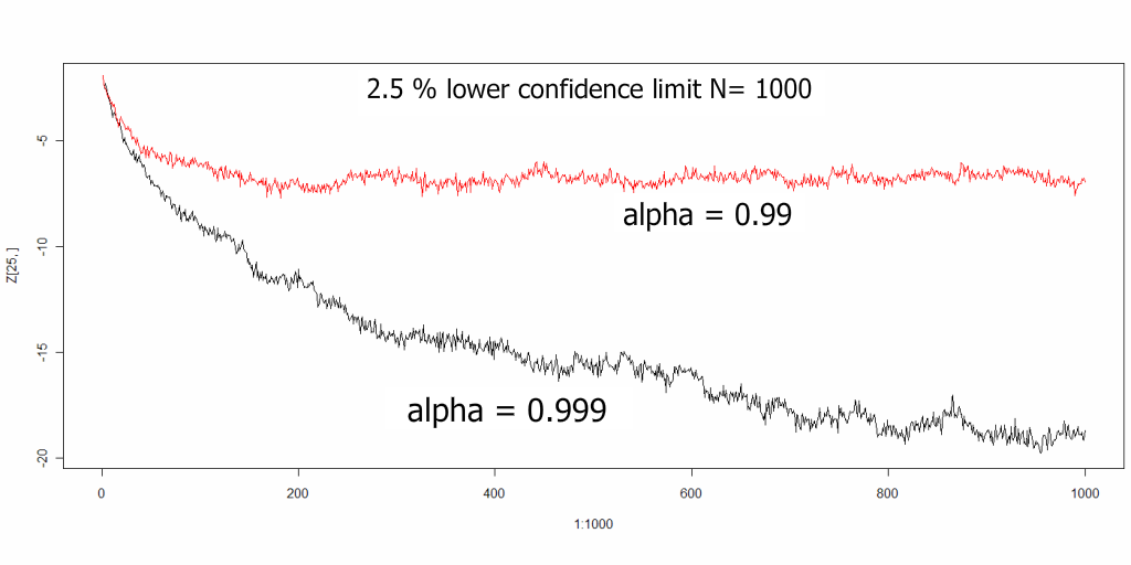
    I expected a difference, but this is pretty spectacular. Note that the difference is apparent even at t=100. I think we have good reason to believe that alpha is less than 0.99 also. Now I have to work out how to plot both sides and put in the temperature series as well. I have little doubt that it will show that the series has wandered beyond the upper limit.

100. Thanks Lucia, that’s helpful. I’m struggling a bit with this because I come from a different background. In my world a stochastic system and a random walk are two very different things.

     I wrote this over at Bart’s:

     Mandelbrot argues that stochastic behavior often arises in systems where large numbers of input variables affect the output and where small perturbations in some of the input variables can lead to large changes in the output. So when many of these hypersensitive input variables are perturbed simultaneously (and out of phase), the combination results in a chaotic output.

     In such systems, infinitesimal errors in assumptions about input variables throw deterministic models completely out of whack. This is why deterministic modeling is often poorly prescribed for many systems. And its why I think attempts at creating deterministic climate models are a fool’s errand.
     —

     I should mention here, that stochastic systems often have damping as well. So that a small perturbation in an input variable can lead to a large change in the output state, but the state can be conditionally bounded (meaning the probability of the output exceeding some boundary becomes diminishingly small — in a physical sense this could mean, for example, that the energy necessary to exceed the boundary rapidly approaches an amount that is unavailable in any realistic sense).

     So in this definition of stochastic, would you still see it as unphysical?

101. In my world a stochastic system and a random walk are two very different things.

     Mine too. Stochastic doesn’t imply there is a unit root. Something can be stochastic, and stationary with no unit root.

102. mpaul

     I should mention here, that stochastic systems often have damping as well. So that a small perturbation in an input variable can lead to a large change in the output state, but the state can be conditionally bounded (meaning the probability of the output exceeding some boundary becomes diminishingly small — in a physical sense this could mean, for example, that the energy necessary to exceed the boundary rapidly approaches an amount that is unavailable in any realistic sense).

     Turbulent flows are dissipative.

     So in this definition of stochastic, would you still see it as unphysical?

     You are describing a class of stochastic systems I consider both physical and common.

103. DeWitt, Lucia

     Koutsoyiannis’s concept of a probability stream tube (see the paper at http://www.itia.ntua.gr/en/docinfo/923/) would seem to be useful/applicable here.

104. PS, Lucia, there’s a nice toy model in Excel there for you to play with as well 🙂

105. Re: Alex Heyworth (Apr 6 19:49),

     I thought the same thing when I saw the result. Now I need to calculate some Hurst coefficients. I haven’t played with the toy model yet.

106. “Stochastic doesn’t imply there is a unit root. Something can be stochastic, and stationary with no unit root.”

     But a cyclostationary process contains a unit root when evaluated over a timescale that is less than one cycle. At a minimum, the glacial/interglacial cycle indicates a non-stationary process – but more likely (allowing for physics), its cyclostationary.

     And there’s a category of complex cyclostationary processes whose periodic component is a linear combination of periodic processes — which would seem very physical to me given that we’re dealing with things like orbit asymmetries, precession, etc.

107. I’ve calculated the confidence envelope for the GISS 1880-2009 anomalies assuming AR(3) and integration factors of 1, 0.999, 0.99 and 0.95 with no trend. I had to offset the GISS data so that the envelopes were symmetric, more or less. Here’s the graph.
     

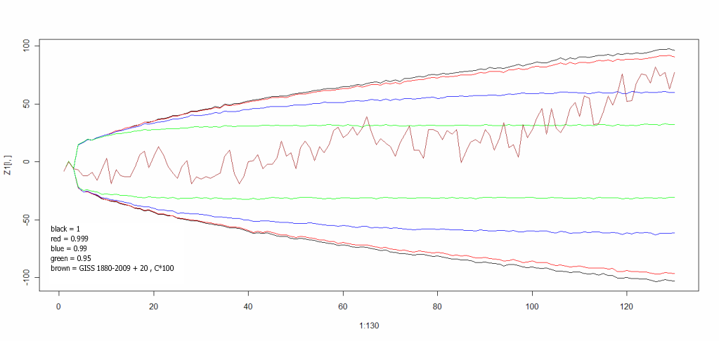
     Again, it’s very possible I’m doing something wrong. But I don’t know what. My unit root confidence envelope looks a little wider than VS’ in the bottom graph in this figure, but I’m not sure we’re using the same AR coefficients. I’m using the one’s calculated for the full series and he may be using just 1880-1935. It still looks to me that there’s a big difference between unit root and near unit root in terms of trend detection.

     

108. Lots of thoughtful comments here, taking the physics into account. Over at my blog the physics minded folks and the stats people don’t seem to find much common ground. Good to see that common ground being explored here.

109. mpaul

     But a cyclostationary process contains a unit root when evaluated over a timescale that is less than one cycle. At a minimum, the glacial/interglacial cycle indicates a non-stationary process – but more likely (allowing for physics), its cyclostationary.

     Question. Does the cyclostationary process actually have the unit root? Or is it simply not possible to reject the unit root given available data? The differences matters.

110. Re: lucia (Apr 6 17:25),
     Lucia, may I reference a couple of comments from Bart’s thread that I think shed a bit of light. A summery from tt

     Here’s another attempt to sum up: The tests for the presence of a unit root in a temperature time series (which VS has performed and no one has successfully contradicted) are for a formal, mathematical property of a data set; it has *nothing* to do CO2 or any other forcing. The conclusion that a unit root is present in a temperature time series does *not* entail that there are no C02 or other forcings. That a trend is “stochastic” (or “random”) does not mean it is uncaused. The presence of unit root simply tells you what kinds of analysis are *statistically necessary* for determining the relationship between data about temperature movements and data about any putative causes of those movements. Failure to follow the statistically necessary methods leads to an invalid, nonscientific conclusion. That doesn’t mean the hypothesis behind the conclusion (e.g. CO2 causes global warming) is thereby disproved. It just means that proof for that conclusion is lacking insofar as it relies on an incorrect method.

     And then Alex

     TT,

     That’s a very good summary! Maybe I could add that in finite samples not only a unit root, but also roots near unity have the same detrimental effects on OLS (this is also pointed out by BV in their paper). So if we get the impression that there is a unit root or a root close to unity, then we should use cointegration.

     Alex

     Finally, this snippet from VS

     Take a unit root process and change the root to 0.999. That’s a “close” stationary process. Conversely, take a stationary process and add to it a random walk with tiny innovation variance. That’s a “close” unit root process.”

     This is the crux of the matter. Cochrane is discussion the theoretical basis for (definitely) establishing unit root presence. Naturally, this is impossible to do, if the AR term is ‘arbitrary’ close to 1, and your sample is finite. However, allow me to quote Alex’s post from yesterday:

     “Maybe I could add that in finite samples not only a unit root, but also roots near unity have the same detrimental effects on OLS (this is also pointed out by BV in their paper). So if we get the impression that there is a unit root or a root close to unity, then we should use cointegration.”

     So, we cannot tell the difference, in finite samples, between a unit root and a near unit root, true. However, the analysis should still proceed on the basis of test results. Cochrane mentions this, and so do Breusch and Vahid. This is important.

     Please excuse the large quotes but I think they are appropriate to the discussion here.

111. Re: schnoerkelman (Apr 7 08:07),

     The question, of course, is how near is near. 0.999 isn’t going to be much different from 1 unless you have thousands of years of data. However, given only 130 years, the difference can be a lot larger than that and still not be distinguishable from a unit root. If I test 10,000 series with alpha from 0.91 to 1, the ADF test rejects the presence of a unit root at the 95% confidence level with the following frequency:

     alpha % rejection
     1.00 4.38%
     0.99 4.75%
     0.98 5.22%
     0.97 5.80%
     0.96 7.34%
     0.95 7.95%
     0.94 10.13%
     0.93 12.18%
     0.92 14.33%
     0.91 17.04%

     A 5% rejection rate is expected if the test is working so an alpha of 0.98 cannot be distinguished from a unit root for a series of length 130. Over 90% of the time, a series with an alpha of 0.95 will test as having a unit root. That’s the green confidence limits in the graph above. All unit root tests have low power against near unit roots when the time series is short. An alpha of 0.95 is equivalent to a time constant of 20 years. You really don’t need a very thick layer of the ocean to get a time constant of that magnitude. If the true alpha is less than or equal to 0.99, a trend in the GISS data cannot be rejected.

112. Lucia wrote:

     Question. Does the cyclostationary process actually have the unit root? Or is it simply not possible to reject the unit root given available data? The differences matters.

     Difficult question. And I’m probably not current enough to answer it. You need to allow for periodicity when testing for unit roots in cyclostationary processes over long intervals. DF can be tricky to apply. Ghysels, Lee, Noh has become a more popular test for unit roots in cyclostationary processes. Unit roots exists at some frequencies and some intervals for cyclestationary processes. In fact, techniques have been developed for identifying frequescies at which unit root behavior can be “averaged out”. But someone more current would need to weigh in. I’m out of my depth.

113. Snorkelman–
     Ok. So in words, what do those quotes mean to anything anyone is doing in climate? And with all due respect to Alex– why does VS finding a unit root in a curve fit mean any one has to use co-integration? Most people don’t do curve fits at all. So, we are supposed to use co-integration to do…what?

114. Lucia

     I guess you’re supposed to use co-integration to do co-integration analysis and find out what drives the temperature.

115. I think what I’ve been doing is determining the type II error, that is failing to reject a unit root when one isn’t present. Out of curiosity, I extended the calculation. The alpha value at 50% rejection is between 0.81 and 0.82 and the 95% level is 0.59. The test becomes more powerful as the length of the series increases, but we’re not going to see 1,000 points. How much better will it be in another decade? At 140 points, the 50% point is between 0.83 and 0.84 while the 95% level is 0.63, so not really any better.

     Now I really do need to find a package that will calculate a Hurst coefficient. Maybe the one that does Fractional Gaussian Noise will work.

116. DeWitt,

     a couple of points: for the ADF test you are performing above, I think you may find that econometric text books suggest different significance values for different sample sizes. I am on holiday, so I can’t look it up for you.

     On Hurst coefficients, I posted at Dave Stockwell’s yesterday on packages with this function available http://landshape.org/enm/hurst-coefficient-software/. The good news for you may be that R has it available.

117. Lucia, first let me state that I’m not in any way qualified to discuss the correctness of the math involved but I feel I “overstand” what VS, tt and alex are saying. An analogy:

     If someone says “I want to measure the temperature of a gas” the first tool many would suggest would probably be a mercury in glass thermometer. This would be an appropriate choice in many cases. But it would not be appropriate if the gas in question was helium surrounding a pipe containing liquid oxygen, nor for O2 being blown into a steel furnace.

     I think this is the point VS is trying to make: the first question that must be asked is what the appropriate method(s) are given the characteristics of the data under analysis. If you find that the data exhibit certain characteristics then some methods are simply not appropriate and will deliver invalid results if used.

     To this: “So, we are supposed to use co-integration to do…what?” I have no idea and do wish VS would get on with it and tell us.
     I would like to make two observations though.
     1) Frequently I see comments that accuse you of semantic games. I have never been convinced of this but rather admire your attention to detail and precisely specifying the point under discussion. I believe that VS is doing the same thing in this case.
     2) Yes, he does seem to have a healthy ego. No, he is not alone 🙂

     Back to lurking for me!

118. The way I see it is like this. Letting the data do the talking is fine if you have enough data so that your tests have power. And even then, if in doubt be conservative and assume unit root if you think the process is close to containing a unit root. (my terminology is probably wack but…) What I see from Breusch and Vahin (and the Cochrane link that was posted at Barts) is that the instrumental record probably isn’t long enough to just let the data do the talking, and that you have to look elsewhere to see what is going on. So in order to come to a conclusion about what is going on you need to look at the physics. Which takes us back to the conclusion of Bruesch and Vahin again…

     To my mind VS underplays (or even dismisses) the limitations of the tests he has carried out. I think he is in error for doing that, based on the above. He also seems to be saying with one voice that he is just letting the data speak, and then in another voice, saying that if you eyeball his graphs it proves his (3,1,0) correct and better than (0,1,2). It is a strange inconsistancy especially when he is trying to convince people to just rely on the statistical tools. He says that Breusch and Vahin don’t approach the topic of the presence of a unit root when they clearly do. It is getting weird.

119. jk

     etting the data do the talking is fine if you have enough data so that your tests have power. And even then, if in doubt be conservative and assume unit root if you think the process is close to containing a unit root.

     The principle you describe is fine if we really know nothing, or don’t have strong reasons to consider something true even before we have data.

     The problem is this clashes with a rule scientists and engineers follow when in doubt. That rule is: when doing a statistical analysis, don’t make a collection of assumptions that would seem to violate physical principles as strongly believed as conservation of energy.

     To some extent, VS seems to applying your rule of “when in doubt”, using a test with low power, and making a conclusion that seems to violate conservation of energy. Then, even though the low power means there is no evidence that an assumption that violates conservation of energy should be true, the just dives right in and expects people to think those results should sway them.

     As far as I can tell, he just doesn’t want to discuss the physics issue, and wants to decree that we must do it his way because there is no other way. Well… that’s hooey. There is a whole class of statistics called Bayesian that tells us that we are allowed to use priors. Even frequentists statistics lets us decides what power we require to be convinced that a test suggest the null hypothesis really is true. It may well be that his rule is prudent in economics. But that doesn’t mean that rule can’t be discussed. It doesn’t mean people can’t explain why they don’t follow his rule, and will not believe that rule must be given higher priority than “doesn’t violate the 1st law of thermodynamics.”

120. Lucia, I agree with you. There is this big flag in the middle of all of this which is basically.

     “The proper handling of deterministic trends is a vital prerequisite
     for dealing with unit roots.”

     How you do that seems to be more tricky.

     The Cochrane comment http://faculty.chicagobooth.edu/john.cochrane/research/Papers/cochrane_unit_roots_macroannual.pdf talks about “unit root wars.” So i guess there has been (still is?) debate as to the usefulness of the tests. There is langauge in there that echoes Eduardo Zoritas comments at Barts too…

     “This is a dangerous argument, since it implicitly acknowledges that
     unit root tests cannot accomplish the mission for which they were designed, and that mission is not interesting. But it is useful to think about anyway.”

     The paper Cochrane comments on is available as a working paper in pdf too, but I haven’t looked through it.

121. Re: Alex Heyworth (Apr 7 22:04),

     l tried that one. It seems to be designed for looking at random walks specifically rather than time series. I found another one: hurstBlock in the fractal package that looks to be more useful for time series. There are several methods that can be specified for the test. It looks like “higuchi” is the one that produces data that looks somewhat like the plots in Koutsoyiannis’ papers. Much like unit root tests, a long time series produces better results. In that package, a pure unit root series gives H~0.5 and white noise is H~0. I need to crank up K’s toy model to see what that gives for a test result.

     If you set the significance level higher (p value lower) for Type I, don’t you increase the Type II error?

122. Re: jr (Apr 8 09:38),

     Moneywall, groan. However, the first paragraph is interesting. When I posted a comment in the other thread that stated that the unit root tests had low power for short, noisy series, VS replied:

     Do note that these issues have been studied to death in the econometric literature 🙂 However, your effort is appreciated.

     That says nothing about the truth of my statement. It may have been discussed to death, but apparently a lot of of the discussion echoes my position.

123. DeWitt, I see the Cochrane pdf fine from home, the working paper pdf that I am assuming is perhaps an earlier version of the one the comment applies to is here http://128.197.153.21/perron/712/nber-tech100.pdf

     They are both from 1991 so things might have moved on from then ’til now of course.

     For what it’s worth, I think your statement is likely true. My limited reading around the subject seems to bear it out at least.

124. DeWItt,

     http://bm2.genes.nig.ac.jp/RGM2/R_current/library/fractal/man/hurstBlock.html

     I think that might help

125. Re: steven mosher (Apr 8 10:45),

     Thanks, but I’ve seen it. That’s what you get if you enter ‘?hurstBlock’ or ‘help(hurstBlock)’ on the R console after you’ve loaded the fractal package.

     Learning a new programming language is a pain in the ass, especially when I haven’t done any serious programming since graduate school. At least I don’t have to enter the program and data on punch cards and wait hours for them to be run. My current desktop probably has more power than the CDC6600 I used in grad school too.

126. Tell me about Dewitt, learning R for me has been “interesting”

     what would you prefer to use? Matlab? or something else

127. Re: Alex Heyworth (Apr 7 22:04),

     I think you may find that econometric text books suggest different significance values for different sample sizes.

     Ignore my first reply. I usually get things backwards on hypothesis testing the first time around. Obviously you want to increase type I error to reduce type II so you lower the confidence level or increase the p value.

     Another way of looking at it would be to see what would be the minimum level of alpha that would be rejected at the 95% confidence level given the p value found for the series. For adf.test on the 1880-2009 temperature anomaly series with three lags maximum, the p value is 0.45. The corresponding value of alpha that is rejected with greater than 95% confidence (N=5000) is 0.87.

     Re: jr (Apr 8 10:32),

     I was sent to the JSTOR page and I’m not a library or academic institution or JSTOR subscriber. The new link worked. Thanks.

128. For the most part, we expect large persistent changes in temperature to only result from changes in forcing. We don’t expect the earth’s temperature to wander about aimlessly with no preferred level.
     .
     I do not know who the “we” in the above is .
     Clearly this “we” doesn’t include any scientist familiar with non linear dynamics and out of equilibrium systems . And that makes a lot of people .
     Once one removes the word “aimlessly” which is indeed incorrect , “we” fully expect the Earth’s temperature to wander about with no preferred level and this will happen on all time scales .”
     It is even the most basic property of a chaotic attractor .
     That chaotic attractors exist is beyond any doubt , there is a well developped theory (at least for temporal chaos) and the things like the ergodic theory are not new either .
     So yes , the trajectory in an out of equilibrium system in chaotic regime will wander all over the attractor (e.g take different dynamical states) without EVER settling in any “privileged” point .
     The very existence of the attractor which is btw fractal in most cases , is the proof that it can’t be reduced to a point or a small neighbourhood of a point in the phase space .
     Trivially an N dimensional attractor with N finite can be projected on a coordinate axis of the phase space which can be f.ex the temperature .
     It is this projection that constitutes the temperature time series which are discussed here .
     And it is again trivial that this projection has the same features as the whole N dimensional trajectory – typically small variations of any parameter provoke large variations of some (same or other) parameters .
     The analysis of the Lyapounov spectrum will even give the answer on the question which parameter is the most sensible and which is the least . All this is or should be known .
     The added difficulty being that , by definition , very different dynamical states project on the same point (have the same temperature) .
     Drawing conclusion about the ful dynamic of the system by observing only it’s projection on one arbitrary axis (temperature in my example) among the N dimensions of the attractor is shaky to say the least .
     .
     The disturbing point is not that so many people still use linear equilibrium theories on non linear out of equilibrium systems . It’s their problem .
     The disturbing point is that all that has been understood by Poincare already 100 years ago , there is a huge body of important and proven results yet we have in the 21st century still people for whom the very existence and properties of chaotic dynamics is a scoop .

129. deWitt
     Now I really do need to find a package that will calculate a Hurst coefficient. Maybe the one that does Fractional Gaussian Noise will work.
     .
     Just for your amusement .
     We checked with Dan Hughes just out of curiosity the Hurst coefficients in known chaotic systems e.g those defined by a system of non linear ODEs (Dan is a real computer wizard so he does that and more without any package) .
     They are not FGN .
     What is actually not surprising 🙂

130. Tom–
     I agree that my wording is over simplified, leaving out the possibility that the privileged ‘point’ is a more likely an attractor. But what I mean is that the system is not going to take on arbitrary states and just wander around. If forcings are somehow constant, it seems to me there must be an attractor, that is relatively tight compare to “all possible temperatures from 0K to infinityK”.

     I really don’t think the notions of those who use averages, standard deviations and correlations represent any contradiction to the notion that something is chaotic. The issue is simply: When it comes down to brass tacks and we want to try to predict what is going to happen tomorrow (rather than wait for major breakthroughs on the part of the community working on chaos), what tools can we use?

     So, the message of what “physics requires” would be sort of like this:

     
     In the above, I imagine that if (by some miracle) the annual average forcing is constant, we could plot something like [T(t+1),T(t1)] and find an attractor of some sort, like the one illustrated in blue above.

     We’d find that at any time,
     * T(t) falls the range permitted by the attractor. This means the possible range of all T(t) are bounded. Those interested in chaos can now talk to each other about chaos, and its many splendors.
     * Others can observed: If T(t) is at its highest possible value, it will drop; if its currently at its lowest possible value, it will rise.

     * If you watch that process over a long time, for many chaotic systems, there still exists an mathematical average value for T(t) <T>, and the temperatures do cluster around that value even if it’s not a “preferred” value in the sense that some sort of equilibrium is achieved when we encounter the event T(t) =<T>.

     * The average <T> averages may or many not have uses going forward. I think whether or not it’s useful depends on our goal, but at a minimum, <T> is descriptive.

     * People observing the system would note the tendency for temperatures to cluster around that average <T>. We would also be able compute descriptive statistics like standard deviations. If we watched long enough, we would be able to define a correlogram. Some might not think these things are useful or they might not think these statistically descriptive quantities provide the maximum possible physical insight, but they would still describe something about the system to others. (And some people might still use them to predict the next state even if they don’t use the language of chaos. Others might use them to come up with USDA climate zone maps.)

     * In terms of climate change, we anticipate that increasing annual average forcing could shift the attractor like so:

     
     In this cartoon, I illustrate the notion that if the world is held at lower forcing, the temperatures fall on an attractor with a lower average temperature. At higher forcing, they fall on an attractor with higher forcing, so both T(t+1) and T(t) are at higher values than for the other attractor. (It’s plausible the entire shape and form of the attractor could change– but I didn’t capture that notion in the cartoon. It’s a cartoon….)

     But, really, I don’t think the idea of “chaos” and the idea of describing the system using descriptive statistics, or even trying to forecast using the descriptive statistics are that far apart. I don’t think it’s even slightly disturbing that people continue to use statistical tools even though others prefer to think about chaos. In huge numbers of chaotic systems, the descriptive statistics can be defined both using formal mathematics, and, given sufficient amounts of time, we can get decent estimates based on observations. Sometimes these descriptive statistics have some uses, and we can even draw some conclusions based on them.

     In parallel, people who think they can better understand the system using the tools of chaos can do so. The two points of view can interact, and have done so since the time of Poincare!

131. lucia,

     I did some more analysis on the fitted values and residuals from a two box model fit to the GISS anomaly series. The Durbin-Watson test and the Breusch-Godfrey test show that there is still autocorrelation in the residuals. Jarque-Bera, however, fails to reject a normal distribution for the residuals. For the residuals, the ADF and PP test strongly reject the presence of a unit root and KPSS fails to reject stationarity. Testing AR models for the residuals, only the first coefficient is significant (AR(1)). For the fitted data, ADF fails to reject a unit root, but does reject for the first difference. The ARIMA model for the fitted data looks to be (2,1,0), or possibly (0,1,1). Whether all that is sufficient to rule out a spurious fit is still not clear to me, even after reading the Campbell-Perron paper. What did seem clear to me, though, is that finding a unit root (or near unit root) in the time series of interest does not rule out the presence of a deterministic trend because the deterministic trend itself can have a unit root. Just because linear models are used frequently does not mean that one is limited to only considering linear models.

132. DeWitt–
     Interesting.

133. I suggest that many of you, Lucia included, are making a fundamental error in dismissing the presence of a unit root in the temperature series. You all seem to be under the impression that “it cannot be so”, but you are assuming you are dealing with an accurate representation of “the” temperature of the earth.

     Surely a simple solution to the whole issue is that there is indeed a unit root in the data as presented, and that its presence there is related to what is actually being measured. The conclusion is that the data in question is a poor representation of temperature and that some measurement factor is present producing the “unphysical” properties.

     For example, one could postulate an effect similar to UHI contaminating the measured record, UHI would be cumulative and give the appearance of a trend where none really exists.

     Also, with regard to B&R’s paper, showing that temperature is not l(1) but l(0) makes it even harder to show a CO2 concentration (which is so far undisputedly l(2)) to temperature relationship without proper treatment of the data series.

134. Re: Ed Snack (Apr 12 22:24),

     A near unit root looks very much like a unit root over a short time scale. 130 years is short. However there is a large difference between a series with a root that is less than 1 and a root identically 1 as outlined above. A unit root process with a constant input will diverge from zero at a constant rate. Solar radiation produces a constant input. Beenstock and Reingewertz ignore this by only looking at the irradiance anomaly rather than the absolute irradiance. The Earth both absorbs and emits EM radiation. The tank leaks. Therefore temperature, whether we are measuring it accurately or not, cannot be an identically unit root process, but it can be a near unit root process.

135. >>Solar radiation produces a constant input. << This is not correct, expecially at non-visibile wavelengths. Regardless, I see the increasing model instability as resolution is increased as a strong indication that the underlying assumption: >>most of the fluctuation observed in temperature is actually signal, not noise<< is wrong.

136. Doesn’t the GHG model imply a unit root?

     For example, add one extra molecule of CO2 to the atmosphere. This will introduce at step-wise increase in temperature that will not be matched by an increase in re-radiation, except after a permanent increase in temperature.

     This is a unit root. Therefore statistics that are known to deliver spurious conclusions with unit roots should not be used with the GHG model. No prediction is much better than a wrong prediction, because at least you will recognze the risk.

137. AGW refuted?
     Since we know from the physics of CO2 under AGW, an increase in CO2 will result in a permanent increase in average temperature, we know that the temperature record must contain a unit root.
     However, it has seen argued on this blog that the temperature record does not contain a unit root, only a near unit root.
     This is a contradition. The absence of a unit root in the temperature record means the increase in temperature from increased CO2 cannot be permanent and AGW is refuted.

138. Re: ge0050 (Apr 23 13:42),

     But the B&R unit root argument is that since the CO2 data is I(2) (has two unit roots) and the temperature anomaly data is I(1) then a step change in CO2 does not cause a permanent shift in temperature, but a spike followed by a decay back to the previous average, or a delta function in the limit of infinitely rapid response. The solar anomaly data was found to be I(1) and so the temperature anomaly and the solar anomaly were directly related. However, for a true unit root process, a step change in solar, which would be I(0), would produce a constant rate of temperature increase that would continue forever. A near unit root process, OTOH, gives an increase to a new constant level that is approached exponentially for a step change in the input. Near unit root process are bounded and stationary in the long term. A unit root process is a random walks and is not bounded.

Comments are closed.