In comments on David L. Hagen wrote:
H-K dynamics includes persistence with higher fluctuations that is not well modeled in GCMs.
I responded
I’m beginning to suspect GISS Model EH has HK natural variability. I’ll discuss that later. (I’d sent Demetris some “slope-o-grams†that I’d ginned up because of my suspicions about these things. I made the ‘slope-o-grams’ because of questions I had about Model EH, and I’ll be discussing them further later on.)
Steve Mosher then encouraged me to reveal the “slope-o-grams”. I’ve been hesitating because of the need to explain a whole bunch of things related to what I think they show. This afternoon, I posted very disorganized post discussing some language and trying to explain a few reasons why I think these things may be useful for revealing whether the natural variability a particular model is Long Term Persistent (i.e. LTP and/or HK) or short term persistent (e.g. ARIMA, White Noise or a number of other possible unnamed processes.) I’ll now show “slope-o-grams” from computed based on data from some climate models and explain why I suspect the global mean surface temperature GISS Model EH — and some other models– may exhibit HK natural variability.
Computation of Slopegrams
As discussed previously, if I have multiple run created by a specific climate model (or synthetic data) with all runs forced identically, I can compute trends. So for example, if I had 3 runs of 1024 “months” worth of data of some stochastic process whose expected value varies with time, I could compute a 1024 month trend for each of the 3 runs. This would provide a set of (M1,M2,M3) each computed at a scale of 1024 months. Based on these three trends, I could compute a standard deviation of trends at 1024 months, which is an estimate of the variability of computed trends for this period: $latex \displaystyle s_m^{(1024)}(t) $ . This is an estimate of the true standard deviation of trends for the process in question. I previously showed this standard deviation is a function of the ‘natural variability’ or “fluctuating” component of the process and unaffected by the forced portion of the process.
Similarly, to estimate the standard deviation of trends at a scale of 1023 months, I could compute three trends over a scale of 1023 month trends based on months 1-1023 and compute that standard deviation with the start date of month 1. Alternatively, I could estimate based on months 2-1024 with start date of month 2 Both are equally valid choices. To avoid accusation of cherry picking on to get a slightly better estimate than possible from only one choice, I could compute the standard deviation for both and based my estimate of the standard deviation of the trends at a scale of 1023 months on the square root of the average of the squares of these two standard deviations.
I can then repeat this process for a scale of 1022 months, and continue on down to a scale as low a 3 months. This is more or less what I did with white noise– but rather than compute using every single possible start date in an interval (which too hours on my mac) spaced out start dates by a number of years. (For models I used 3 years; for synthetic data I used 60 years. ) The slope-o-gram computed from 7 replicate samples for a process consisting of the sum of a trend and white noise is shown below:

The slope-o-gram shows $latex \displaystyle s_m^{(n)}(t) $ as a function of n in months on a log-log plot.
Since the main purpose of this slope-o-gram is try to detect hints of long term persistence, it’s worth examining this case to identify features that indicate the fluctuating component of this process is not long term persistent. First: notice that I fit a trend of the form $latex \displaystyle s_m^{(n)}(t)= C n^m $ with ‘C’ and ‘m” constants through the data at the largest scales. When the ‘internal variability’ in climate model or synthetic series is short term persistent, the fit will result in a value near m=-1.5 as the number of months approaches infinity. Of course, I will not have an infinite number of years in any data sets, but values of m near -1.5 at higher scales suggest the ‘internal variability’ in a model or synthetic series is short term persistent. The figure above is based on a series whose internal variability is “white noise” which is not only short scale persistent– it has persistence of zero. For that reason, the trend is close to -1.5 at all scales.
Lesson 1 of slope-o-grams: Having a slope of m=-1.5 at all scales is a sign of white noise. Having a slope of m=-1.5 at larger time scales is a sign of short term persistence. Slopegrams for short term persistent process include these for AR1 and ARMA1,1 processes:
AR1: |
 |
Notice the standard deviation of trends for both cases illustrated decay less rapidly with scale at small scales, but eventually follow the m=-1.5 trend exhibited by white noise. It is the behavior at long scales that suggests these are short term persistence. (In this case we know they are because the I synthesized the data.)
Do any models suggest short term persistence?
Some commenters at blog seem to be under the impression that all model show short term persistence in global temperature series. To try to detect whether the internal variability in models might be long term persistent, I repeated the analysis applied to synthetic data to models using model data from 1890-2099. Based on inspecting slope-o-grams I’d say some seem to do so. Two examples are ECHAM and CGCM2.3m, CGCM3_1_t47 and NCAR PCM1. All four show slopes approximately equal to m=-1.5 at the largest scales for which I was able to compute more than two non-overlapping sets of trends for each run. (That is: 83 years.)
 |
 |
 |
 |
Long term persistence
Processes with long term persistence will be characterized by displaying slopes of between -1.0 and -1.5 at long time scales. Ideally, to detect long term persistence requires access to infinitely long time series, but my computations were limited to data from 1890-2099. Based on these series, the following AOGCM’s appear to exhibit long term persistence: FGOAL (wow!), GISS EH, GISS ER, GISS AOM, NCAR CCSM and ECHO-G.
 |
 |

|
 |
 |
 |
Notice the trends decay less rapidly than m=-1.5 at large time scales. This is suggestive of long term persistence or Hurst-Kolmogorov behavior. I’m not going to say it’s proof– it would be nice to have longer time series, but it is suggestive.
Owing to the past hot arguments about the possibility of non-stationary series, I’ll note that:
- Some models are showing m~-1.0 at the larger time scales; one actually shows m=-0.98. m=-1.0 represents the boundary for stationarity. My view — based on physics– is that all are likely stationary and the value of m=-0.98 is the result of either close to non-stationary behavior combined with lack of resolution (owing to having only 3 realizations) and too short a time series to detect the asymptopic behavior.
- No model shows m~-0.5, which would be associated with first differencing in ARIMA. I believe that such a slope would violate our understanding of radiative physics and the first law of thermodynamics.
- For those who think that LTP or HK by itself automatically means that we would be able to decree earth trends are consistent with with natural variability: Nope. In all models, the standard deviation near 83 years (or larger numbers of years) would safely ensure that the magnitude of earth’s trend fit to data could safely be decreed statistically significant if we accept any individual models estimate of the variability of 83 year trends as correct. (This means nothing if you believe absolutely nothing from models.) This is true even for models that seem to indicate long term persistence.
Long term persistence does not not necessarily mean that the variability of 100 year trends is extremely high. Some long term persistent models have relatively low variability of short term trends. So, while it is true the variability in trends persists– that is it does not decay at a rate of m=-1.5, it is not particularly high.
I’m not sure what more I can reveal about LTP in models. This analysis was something of an exploratory analysis– but Steve Mosher was interested in seeing the hints of HK I think I am seeing in climate models. This is pretty much it: The “slope-o-grams” for some models may decay too slowly to be Short Term Peristent. At least based on these slope-o-grams, if someone suggests HK doesn’t appear in models, I would ask them to explain the basis for their opinion because some models seem to exhibit HK in the surface temperature series.
Ha, Thanks. Gosh, A long while back when Dr. K was hanging out at CA, I was wondering if we could score climate models by looking at the hurst coeff of the output and how well it compared to the husrt coeff we might see in the observations. Just a concept of a different sort of metric for a simulation being “realistic” I was drawn to that because obviously one doesnt design a simulation to have a specific hurst coeff in the output.
Mosher, “Dr. K” did exactly that in a recent publication:
Anagnostopoulos, G. G., D. Koutsoyiannis, A. Christofides, A. Efstratiadis, and N. Mamassis, A comparison of local and aggregated climate model outputs with observed data, Hydrological Sciences Journal, 55 (7), 1094–1110, 2010.
http://itia.ntua.gr/en/docinfo/978/
The result was that the models systematically underestimate the hurst coeff (and also std).
Lucia, are you aware of Haslett (1997)? I think you might find it interesting.
Haslett, J. (1997) On the sample variogram and the sample autocovariance for non-stationary time series. Statistician. 46, 475- 484.
Wow!
Time-out for a bottle of wine (NZ Sauvignon Blanc, since you ask) and a sleep and there are 3 new HK-related posts! I suppose I must thank Mosh for stirring things up.
Lucia, ‘So for those thinking yesterdays post is a claim that internal variability is not LTP – that was not my claim. I am simply showing that the “climograms†of RSS are not particularly good evidence of LTP when the prevailing notion is that the data contain a trend’, sorts out all (well, most) of my issues.
Apologies for the ad populum comment – I now see from whence you are coming.
Sorry about the formatting – only the initial ‘not’ was meant to be emboldened.
Mosher
I don’t know how you can get the actual hurst coefficient for the surface temperature over the 20th century. If the 20th century contains a trend, the hurst coefficient from a climacogram will look higher than it really is because it will be polluted by the trend.
JeanS–I’ll look at Haslett. I’ll look at that DK paper too. But… it seems to me that lots of these papers examine things under the assumption there is no forced trend. The difficulty is if it really is there– and if our question is really to determine if it is or is not there, I’m pretty sure that simply assuming the time series does not contain a trend there will always make Hurst coefficients look to large. Just detrending by assuming linear doesn’t help much either.
[quote]I don’t know how you can get the actual hurst coefficient for the surface temperature over the 20th century. If the 20th century contains a trend, the hurst coefficient from a climacogram will look higher than it really is because it will be polluted by the trend.[/quote]
Wouldn’t that apply to the models also, so you are really comparing apples to apples?
[quote]things under the assumption there is no forced trend[/quote]
IMHO, you are reading too much to this self-constructed “forced (non-linear) trend” -issue. This is not to say I necessarily believe the LTP-model is correct for the temperature series.
JeanS–
I’ve concocted an idiosyncratic method with these slope-o-grams. It’s insensitive to the functional form of the forced component but requires replicate realizations.. We can get replicate realizations for the models because some have multiple realizations. We can’t get this for the earth because we only have 1.
If I could get a slope-o-gram of the sort shown above for the earth, I would– but I can’t.
As for whether we can compare the output of the same statistical process applied to the earth and to models: Sure. That’s apples to apples. But I still think we can’t know the hurst process for the earth’s time series.
Jean S–
The Koutsayiannis paper is here:
http://www.informaworld.com/smpp/content~db=all?content=10.1080/02626667.2010.513518
Interestingly enough, the Hurst coefficients for the earth are compared to ECHAM, PCM, CGCM ahd HADCM3. Note my table of “not hurst” examples for models includes “CHAM and CGCM2.3m, CGCM3_1_t47 and NCAR PCM1”. (There were no replicate samples of HADCM3, so I don’t know if that one looks like HURST.)
So, by coincidence, it appears Demetris’s comparison of Hurst coefficients is to the models whose surface temperatures happen to not look Hurst by my method.
He doesn’t happen to compare the observed Hurst parameter to those in “FGOAL (wow!), GISS EH, GISS ER, GISS AOM, NCAR CCSM and ECHO-G.” whose surface temperature series look like might be very Hurst-like.
I’m also not sure whether his method of downscaling might not automatically reduce Hurst coefficients– but I’d have to think a long time to figure that out. The issue of comparisons to the “non-Hurstian” collection of models strikes me as possibly meaningful. (Note: I don’t think there was any way for him to know in advance which are “Hurstian” and which “Non-Hurstian”, but it still may matter.)
You seem to have put a lot of work into this!
.
So if I understand correctly, some models’ outputs for 1890-2099 appear to show HK behavior, which is to say, some models do appear to contain variation on multiple, fairly long time scales, while others do not. Which suggests that some models are better at replicating the kinds of natural variation that DK notes is present in a wide range of natural processes. OK.
.
But I have two doubts.
1. We know that climate modelers are quite aware of the actual temperature history from 1890 to 2000, and we know that some models incorporate forcing from volcanic aerosols and others do not. I wonder if those models which incorporate estimated volcanic forcings (and man-made forcings?) to better match the temperature history are the self-same models which appear to have more natural (that is, HK) behavior, and the models which don’t include estimates of volcanic aerosols are the ones which don’t show HK behavior. I guess what I am saying can be summarized as: “Forcing” a match to the historical temperature data with assumed historical aerosol forcing patterns will automatically yield the same type of “natural” statistics as the historical pattern. If projections out to 2099 include random volcanic eruptions, then even model projections would have those same statistical characteristics.
.
If the models do not include random volcanic forcing after 2000, and the 2000 to 2099 periods has the same HK behavior, then that might be more convincing.
.
2. If we believe that long term temperature variation, as evident in the MWP-LIA-modern warm period variation, is real, then that should also be simulated by the models if run for a long enough period. If we believe that those kinds of long term variation are in fact causal, then the physical mechanism(s) which create those long term variations would have to be included in the models for them to credibly predict climate behavior on very long time scales. I very much doubt that is the case.
Naive question — You’ve been considering GCMs and their characterization of climate as far as persistence (e.g. H-K long-term persistence, various flavors of ARIMA for short term persistence).
Clearly, model builders can declare, “We want our GCM to have a Hurst coefficient of X (etc etc), because we think that reflects the physics of the actual climate.”
On the other hand, to what extent can such properties be “emergent”? In those cases, a GCM could exhibit a given property in the absence of intention on the part of its builders (and, equally, in the absence of knowledge of such properties).
I believe that the answer is analogous to that for “nonlinear dynamical systems” (Wikipedia cite) — “Either scenario is possible.” If this is not correct, I’d be interested in an explanation.
JeanS
.
IMHO, you are reading too much to this self-constructed “forced (non-linear) trend†-issue. This is not to say I necessarily believe the LTP-model is correct for the temperature series.
I also tend to see the matters in this way.
This whole discussion reduces to the following dilemma :
1) I have a time series Xi which has a property Px (f.ex HK or deterministic chaos or …)
or
2) I construct 2 time series Yi and Zi such as Xi = Yi + Zi . Yi and Zi have properties Py and Pz .
Once formulated this way , it appears clearly that there is no statistical test which could say whether 1) or 2) is preferable let alone true .
IMHO 2) seems to contain to many more or less arbitrary and probably unnecessary assumptions so in a general case I’d prefer 1) which is much simpler .
This doesn’t exclude of course some exceptions where 2) would be better but I’d need a very compelling (e.g non statistical) argument to abandon 1) for 2) .
I would also suspect that as there is an infinite number of possible series giving the same sum , 2) could give an artificially good fit .
.
Lucia
.
I appreciated when you reminded vortex shedding in the other thread . I was just about to write a comment talking about vortex shedding when I found yours so it spared me time .
Is this getting to depressing?
+0.13C May? Not posting UHA anymore?
Annabelle–
Interesting question. But I’m always willing to provide TMI when people ask a certain post isn’t out. I wanted to finish this up when I learned the UAH was posted. Owing to a scheduled colonoscopy today, I wasn’t really able to do much after 8pm last night. I was rather occupied by responding to the effects of “Movi-prep”. I’ll be posting UAH after taking a nap.
Out of curiosity, what do you think is depressing about the UAH data? that’s it’s trend remains quite a lower than projection suggesting warming is slower than modelers suggest it should be? Or something else.
SteveF–
It would if my “slope-o-grams”were computed based on single series. But the effect of forced response should out when I compute over multiple series. (I’ve done test by puting sinusoids in the determinist part and it has no effect on the results.)
A Mac
You can ask Gavin since some of this is in his models. I suspect the HK is emergent, not snuck in.
Tom Vonk–
Huh? There can be statistical tests to say whether (1) or (2) is preferable.
I don’t think saying a system can be divided into “mean” and “fluctuating” componenets is particuraly complicated. In anycase, even Koutosayiannis does this. He just likes assume that the form of one of the function is “mean value, not a function of time”. In contrast, my assumptoin is “the function exists” (but the possible forms include mean value, not function of time.)
So I’m the one making fewer assumption.
In anycase, if the only goal is to detect whether or not a a deterministic portion exists, it is rather odd to simply suggest the general principle is to use a model that ignores it’s presence at the outset and assume whatever deterministic portion exists must be part of the natural variation. The latter method will always inflate our estimates of natural variability– and since the mean was used in estimating it’s magnitude, you will nearly always find a way to suggest the mean falls inside the range of uncertainty. It almost must if your estimate of uncertainty includes the variations due to the mean!
Apologies re your op. Meant that even lukewarming has stopped
heres some real long term persistence
http://www.youtube.com/watch?v=zEQ79hE-Uo0&feature=player_embedded
Laura– No problem. That’s just the reason for the delay. I went and took a nap– as advised by the physician. (Plus, I think the anesthesia hasn’t worn off.)
Here’s the youtube:
So we were 1/2 way to the next ice age in the 70s? 🙂
Re: lucia (Jun 8 12:15),
“Stopping the Coming Ice Age” (1988)
1:42
“But the climate cools so suddenly that agriculture almost instantly becomes all but impossible in most regions of the Earth. Some recent evidence suggests that we may be more than halfway through such a rapid, perhaps less-than-20-year transition period! And that we may be less than seven years away from the beginning of the next Ice Age!”
Lucia,
.
I assume you mean “average out”, not “out”. In any case, I don’t think that addresses the issue. If the (repeated) runs are based on the same assumed set of volcanic aerosol forcings, then the same statistics should (I think) be evident in each case;averaging would make no difference. There is a simple test: which of the models assume volcanic forcing variation (according to the 20th century record) and which do not?
SteveF==”cancels out”.
Yes. I mean the forced trend cancels out.
I’m not sure I know what you mean. I suspect you imagine I am doing a process to run 1, then run 2, then run 3 and averaging or something. I’m not. But maybe you can clarify what test you think I would be doing.
In a model given model, volcanic aerosols are forcings are applied uniformly to all runs. So the response to Pinatubo is a “forced” response in that model and the forced component of the response will appear in all runs of that model.
So consider the computation of the 20 year trend from 1980-2000. Pinatubo blew during that period.
Compute all of these from GISS EH;
Trend 1: M1.
Trend 2: M2
Trend 3: M3
If you feel like it compute the average M_ave. This is affected by Pinatubo. This value also does not appear in anyway, shape of form in the slope-o-grams. It isn’t even computed.
Now compute the standard deviation over the three trends.
I am assuming this standard deviation is not affected by the eruption of Pinatubo. This is an important assumption– as one could argue maybe El Nino/ AMO/ Etc. type “noise” is strongly affected by eruptions, but I assume not. (I don’t discuss this in the current post, but I feel comfortable with the assumption that the standard deviations are not affected by the mean trend because
a) there is no strong reason to suspect the forcing must affect the standard deviation across runs and
b)past test of the standard deviations over different periods suggest the standard deviation of trends across runs do NOT differ from period to period. Note that (a) would not be sufficient to make the assumption because once could argue the forcings might affect the El Nino, AMO etc. That’s why I require testing over non-overlapping periods to see if the standard deviations do vary over time. They don’t. Of course in a full paper I would have to collate all of these things in one place– but this is a blog post.)
Oh. FWIW: With synthetic noise, I’ve added “weird” forced trends to all runs. That is:
Create synthetic run 1.
Create synthetic run 2.
Create synthetic run 3.
Make “slopeogram 1”.
Add “cosine(omega T)” to all three runs. That is: Add the same forced trend.
Make “slope-o-gram 2”.
The two slope-o-grams are exactly the same.
This is property is not shared by DK’s climacograms. That’s because with climacograms, the best I can do is make a climacogram for run1, a new one for run2, a third for run 3. Then I average the three.
With my slope-o-grams, I cannot make a slope-o-gram if I only have 1 run. Can’t be done. The “cancel out” has to do with taking standard deviations across matching periods of runs.
AMac– We were only 7 years away. Amazing, huh?
Hi Lucia,
Here are the model descriptions, in terms of forcing agents:
.
All models include green house gas forcing (GHG) and direct sulfate (SD) forcings. Other forcings are:
SI – sulfate indirect
BC – black carbon
OC – Organic carbon
MD – Mineral dust
SS – Sea salt
LU – Land use
SO – Solar intensity
V – volcanic aerosols
.
No long term persistence:
MRI-CGCM2.3.2 – SO, V
ECHAMPS5 – O, SI
CGCM3.1(T47) – none
NCAR-PCM1 – O, SO, V
.
Long term persistence:
FGOALS – none
GISS Model EH – O, SI, BC, OC, MD, SS, LU, SO,V
GISS Model ER – O, SI, BC, OC, MD, SS, LU, SO,V
CCSM3_0 – O, BC, OC, SO, V
GISS AOM – SS
ECHO – G – O, SI
.
There is no obvious pattern. I guess you would need to look at each model’s assumed set of forcings to see if the behavior of each model is “inherently” persistent or the result of a contrived set of forcings. Since all three GISS models fall in the same group (persistent), I imagine there is something consistent that makes there models behave similarly.
.
I note that the different models have vastly different variability at different time scales, independent of if they have long term persistence or not.
Lucia,
Based on what you say, I clearly do not understand what your slope-o-grams are/are telling us.
I will re-read.
Ugh,
Been there, done that. Best to have at least two bathrooms and a “keep out” sign.
But on the positive side, climate scientists are always there to help.
http://climateaudit.org/2011/06/08/built-like-an-outhouse/
(Hope your test went well.)
Re: lucia (Jun 8 15:06),
nitpick: Of course the average is computed, you can’t calculate the standard deviation without calculating the mean, at least in principle. But by using only the stdev function, you never see the mean.
Lucia
Appreciate your effort.
My comment was based on the conclusions of Anagnostopoulos et al. 2009 Credibility of climate predictions revisited European Geosciences Union General Assembly 2009, Geophysical Research Abstracts, Vol. 11, Vienna, 611
(After peer review this work was published as:
Anagnostopoulos, G. G., D. Koutsoyiannis, A. Christofides, A. Efstratiadis, and N. Mamassis, A comparison of local and aggregated climate model outputs with observed data, Hydrological Sciences Journal, 55 (7), 1094–1110, 2010.)
That performance did not impress me as justifying spending $1,900 trillion/degree to “control climate”!
I understand your trends to show HK like behavior, but read Anagnostopoulos et al 2009 to describe very poor prediction of HK coefficients. Does evaluating actual values vs anomalies impact the comparison?
Based on what you say, I clearly do not understand what your slope-o-grams are/are telling us.
I thought they simply show the speed of convergence in trend. Take a lot of timeseries generated by a given process – how much do the trends differ from each other after generating X timepoints?
I wonder if some strongly non-stationary processes could generate horizontal slope-o-grams? What’s the slope-o-gram of brownian motion (cumulative Gaussian noise)?
Being very bored, I actually answered my own question. Cumulative white noise strongly reduces the slope (wrt plain white noise), but does not create a horizontal line.
However, cumulative Cauchy noise generates some funky slope-o-grams which do seem to bounce around a horizontal line.
Lucia
I don’t think saying a system can be divided into “mean†and “fluctuating†componenets is particuraly complicated.
I didn’t say “complicated” anywhere because it isn’t .
I said arbitrary and probably unnecessary because it is .
Writing a variable under this form is just a change of variable and there is an infinity of variable changes . You pick up one , you can pick up another .
.
As for the statistical tests .
I will just take 2 among an infinity of variable changes .
1) X(t) = P3 + u(t)
2) X(t) = P1 + u'(t)
P3 is a polynomial of 3rd degree and u(t) is a residual .
P1 is a polynomial of 1st degree (a straight line) and u'(t) is residual .
With what statistical test do you find out which is “preferable” of 1) and 2) knowing that the only variable that can be measured is of course X(t) ?
This is not a rhetorical question .
David L. Hagen
Someone else pointed to that. I have a few comments:
1) The general issues with models (poor efficiencies etc.) aren’t particularly relevant to our discussion on this post. Without reading Demetris’s paper, we know the absolute values of temperatures in models aren’t good because the models disagree about the global surface temperature with each other. So I’m not going to discuss that aspect of that paper except to say that even without Demetris paper, we know the models aren’t good at finding the global average for surface temperature so it’s hardly surprising the efficiencies are bad individual points. Since this post is about Hurst I’m going to only engage the Hurst aspect of implicit in this question “Does evaluating actual values vs anomalies impact the comparison [in Koutoyiannis’s paper]?” instead of going off on a tangent. (I’m also not going off on the tangent of whether we should do anything about climate–we are discussing whether models do or do not capture Hurst.)
.
2) I noticed that the selection of AOGCMs models Koutsoyannis looked at happen, by coincidence to be the models that — based on my climatograms– do not seem to exhibit Hurst behavior in global temperature. Possibly, if the comparison of Hurst coefficients in models and observations had been made to models that do show Hurst in surface temperatures, he’d make a different conclusion about whether climate models over or under estamate the correct Hurst at points. I don’t know– and I’m not going to compute the Hurst at local points from models like GISS EH etc. to find out. That said, knowing the AOGCM’s that show Hurst at large scale are left off, the answer to your question is: Yes. My comparison impacts his because his comparison of models to observations to the subset of AOGCMs didn’t include the models that show Hurst at large scale in his comparison.
.
3) I don’t know whether I would expect downscaling from AOGCM’s to really capture correct the spectral properties at a point anyways. So, the reason for AOGCM’s mismatching Hurst computed based on observatoins might not be the inaccuracy of the AOGCM’s at large scale, it could be that you don’t get that property properly when downscaled. (It seems at least one reviewer must have suggested something of this sort to K. While K’spaper was published, this doesn’t mean the reviewer was incorrect. This is an unknowable based on information available.) It’s possible his comparison could ever tell us much about AOGCM’s ability to capture Hurst coefficients at scales comparable to grid sizes or higher.
.
My analysis adds information because I’m showing that at least some models show Hurst in the variable that averaging scales modelers claim AOGCM’s are supposed to capture has their most robust prediction: Global Surface Temperatures. (Whether models get the “correct” Hurst, I can’t begin to say. I’m not sure it’s really possible to compute the correct Hurst coefficient based on earth data. )
.
4) It could be the difference in Hurst coefficients and earth coefficients presented in K’s paper does represent a difference attributable to some difference between models and observations. But that doesn’t necessarily mean it’s an important deficiency in models. The difference may arise because of something not taken into account in models (and which may or may not matter over the long term and which barely affects the global average temperature) Over times scales of modest lengths (i.e. 30 year, 60 year etc), it’s entire possible that the trends at measurement stations could be affected by changes in local micro-climate induced by things like urbanization or de-urbinization. If so, this can affect the computed value of temperatures at those stations biasing those temperature relative to temperatures in the average in the AOGCM grid cell. (I think Anthony Watts has suggested this sort of thing can happen.)
Models don’t include local changes in urbanization within a grid cell. If urbanization (or just site degradation and improvement) happens and is strong enough to have an even miniscule effect on the average global surface temperature, it seems to me it would have an amplified, possibly very, very strong effect on the computed HURST coefficients at points. This is because while an excess positive trend at site 1 would along with excess negative trend at site 2 would off set each other in computing the global surface temperature, both would result in excessively high computed Hurst coefficients.
.
So, the difference between the observed and model might be because the value computed based on observed temperatures at points are biased high owing to micro-climate issues.
======
Now for my general reaction: In all, I think that paper is an interesting, useful publication.
* I’d guess the specific AOGCM’s Demetris compared to data probably don’t predict Hurst at points– the don’t predict it in global surface temperatures. But that’s because the models that do predict Hurst at large scales were not included in his comparison.
*I think it’s possible his estimate of the true Hurst in the observations may be biased high.
*I don’t know that the paper gives us conclusive evidence about any individual models ability to correct capture HURST coefficients, or even what Hurst coefficients are at the observed points.
* I think what we learn from that paper is: There may be Hurst behavior in the observations. The models that don’t show Hurst at global scales show low Hurst at points after downscaling using the method Demetris used. Maybe those models don’t show appropriate Hurst values– or maybe they do.
* We know without reading Demetris papers and without comparing to observations that the models disagree with each other on Hurst values for global surface temperature– so at least some models must get Hurst wrong.
I know there will be other who think the paper permits us to make firmer conclusions– but I don’t think so. I think it’s interesting, publication worthy, but I don’t think it tells us much about whether all models fail to capture Hurst behavior similar to that on earth. It’s true some models don’t– but for all we know some may.
Tom Vonk–
I don’t know what you mean by “arbitrary”. The expected value is the value that results in E(u)(t)== 0 at all (t). Other choices don’t. It is the choice that partitions forced components — if they exist– from unforced. If no forced component exists, my choice of partitioning results in
Your alternatives don’t have this property for cases where the forced component is zero. So your alternatives
a) can’t isolate the natural variability when the forced component does exists and
b) will give an incorrect value for properties of the fluctuating componenet when the forced component does not exist.
Mine does the opposite on both (a) and (b). So, if someone is interested in learning the properties of the fluctuating component — that is, anything about the properties of x(t) (including magnitude of moments, spectra etc.), it is clearly better that your alternatives. Sometimes we will be able to learn something about some of the moments– sometimes we won’t have appropriate data to learn some other property. But this division permits us to isolate the ‘natural variability” form the mean and other divisions can’t.
Whether or not this partitioning is ” arbitrary and […] unnecessary ” depends whether or not one considers it desirable to tease out the properties of the actual, honest to goodness internal variability from mean forcing. Of course, if you don’t want to isolate properties of internal variability from the forced component and only want to treat the whole thing as one big smeared thing, separating them out is “unnecessary”.
But, to go to analogy space: If one wants to make a souflee, you need to separate the yolks from the whites. If one wants to make scrambled eggs, it’s ‘” arbitrary and […] unnecessary ” ‘ So, I say to you: If you want to make scrambled eggs, go ahead. I love scrambled eggs. But those who want to make souffle’s will find it necessary and desirable to separate eggs from yolks and your intimating that it is it’s arbitrary because– possibly, I could also have concocted some recipe that (for some mysterious reason) mixed the yolks from egg 1 with the white from egg 2, and the yolk from egg 2 and the white from egg 1– and it’s just some sort of arbitrary choice to collect yolks with yolks and whites with whites– …. yeah. I’m just doing it the way I need to do it if I want to collect together “like” things with “like” things, in a way that permits me to have a specific type of product. Which product you don’t seem to value.
But yes– I want to find methods to tease out the forced component from the natural variability– if the forced exists. You don’t seem to value this goal and so think the partitioning is arbitrary and unnecessary and prefer methods that would make us unable to detect the forced component even if it exists.
Lucia
Thanks for your lengthy comments – appreciate your focus on Hurst behavior for this post. Reflecting on:
Poor oscillation tracking: It appears my comment on underestimating persistence or HK behavior, would more properly be that all the models tested by Anagnostopoulos et al. 2009, underestimate ALL major oceanic/atmospheric oscillations. Consequently both the HURST coefficient and the standard deviation are underestimated. To improve this, I presume that the climate models would need to characterize PDO, AMO, ENSO etc etc. Doing so would improve both HK and the standard deviation performance.
Relative performance: Given the poor modeling of ocean/atmospheric oscillations by all models, Anagnostopoulos’ data on differences (eg 74% HK and 70% SD) might still indicate that the models tested do worse on persistence/HK than on short term response/SD. e.g. see Slide 9. 17, 18.
I’ll defer to your expertise on statistics over that.
How does it follow that models underestimating major oceanic or atmospheric ossillations means the honest-to-goodness Hurst coefficient is under-estimated in the earth? (Real question because I’m pretty sure that I can show that if long time constant oscillations are present — and they are really peaks in the spectrum– computing the Hurst coefficient using a time series shorter than than the time period of the oscillation will result in an estimate of the observed Hurst coefficient that is much too high.)
Moreover, DK’s analysis computes the Hurst while neglecting scales longer than 1/10th the full length of the time period T (which I think is his practice based emails), then if he has a 100 year time period, and oscillations with periodicities greater than 10 years even exists his climacograms will over estimate the observed Hurst coefficient for the real process. (I’m pretty sure can show this and will if people want to see.)
So, I think it’s better to observe that all models under estimate major oceanic and atmospheric oscillations and just stop right there without proceeding to looking at Hurst coefficients. Wrong on this is wrong, why confuse things by comparing Hurst coefficients?
I think it would be better to just end by just discussing the standard deviations and forgetting about the Hurst coefficient.
toto–
Sorry I didn’t respond sooner. Random walks (i.e. cumulative white noise) should get a slope of approximately -1/2. It’s noisy though so you probably need lots of runs.
I assume integrating twice will reduce the slope further.
The theoretical trend for white noise is -1.5 because the standard deviation of the mean over N points white noise goes as sd_u= 1/N^0.5 and, but the uncertainty in trends over N points goes as sd_u/N so that’s N^-1.5
The standard deviation of the mean over N points for a random walk is sd_u=N^0.5 — that is it increases over time. But the standard deviation for trends is sd_u/N ~ N(0.5-1)=N^-0.5.
If you have “noise” whose standard deviation over N points increases more rapidly than N^1, the slope-o-gram could show increasing sd with N. I’d suggest there are wildly unrealistic for internal variability. Certainly we aren’t seeing any suggestion of it in models.
Lucia
With all the issues you have identified and analyzed, you have the prospects for a good paper comparing the accuracy of evaluating HK/persistence compared with SD for different models, as a function of the spectra of trends/fluctuations, versus the duration of data analyzed etc. I wish you well with it, and look forward to your further posts.
David–
I’m not entire sure what there is to discuss in a paper. The models do show Hurst. We can’t compare it to observations. So.. what?
Other than DK, what team cares about Hurst in global surface temperatures?
What paper do you thing is worth writing? What point to do think it should be addressing. Because honestly, I don’t see a paper here. But if you thin there is on: suggest what the major point of the paper would be.
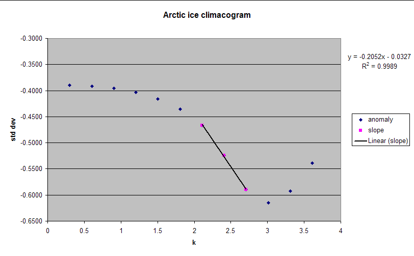
Re: lucia (Jun 9 11:15),
I think I know what you mean. I just did a climacogram for Cryosphere Today Arctic ice area daily anomaly. I used the first 8192 points and there’s a clear reversal in slope at large scale that is too large to be the uncertainty in the standard deviation because of too few points. But a trend would do exactly that. It looked like it was going to be Markovian until the slope reversed (graph here). A graph using the last 8192 points would probably be even worse as the loss trend is larger for the most recent data.
Re: lucia (Jun 9 20:02),
It might be worth at least sending a note to Gavin Schmidt. The fact that some models, including GISS models, appear to show long term persistence and some don’t might be interesting to him. Or not. But you don’t know unless you ask. I’d ask him, but it’s your work.
Dewitt–
I made synthetic graphs like that. The drop can be introduced by a strong cycle. The drop happens close to the period of the cycle. sent graphs like those to DK. Later, the trend shows the uptick.
I’ll send a note to Gavin to see if he thinks anyone thinks this is interesting. I don’t know if he reads my email. 🙂
Re: lucia (Jun 10 06:34),
If you don’t get a reply, I can try. He’s responded to questions from me before.
I did the plot for the last 8192 points and included it with the first 8192. As I suspected, it is indeed worse. It looks like if the trend is big enough, you get something that looks more and more like LTP.
Did you try a linear trend? Since the base unit is days for my graph, I don’t think what I’m seeing in the ice area climacogram is a cycle with a period of 1,000 days. The trend in ice area isn’t linear, but if it’s cyclic, the period is a lot longer than 22 years.
DeWitt–
He’s responded to me in the past. But I sent once– more recently, sent an email and got no reply. So, I thought “maybe he hates me and won’t read my email anymore. “. 🙂 Of course, there are many other likely possibilities. (Spam filter at it, he actually has a life got busy and didn’t answer etc. I’m pretty sure there are two emails in my “inbox” I mean to answer and I haven’t. ) I don’t make a habit of bombarding people with email unless I have a real question, so I wasn’t going to ‘test’ my theory that gavin might now hate me and not answer by pestering to find out why he didn’t answer 1 not very important email. So, the theory remains untested. 🙂 (I don’t even remember what the email question was about. It wasn’t Only that I sent one and got no answer. It wasn’t hellashiously important so… that was that.)