PeteB was trying to puzzle out why I am saying the multi-model mean is outside uncertainty intervals of any ‘best’ ARIMA(p,0,q) model with p<5 q<5 even though last year, Tamino said it was inside the uncertainty intervals for ARIMA(1,0,1). Specifically he asked:
luciaI was just interested in how noisy these relatively short periods are
When I look at here from Tamino’s (albeit a year ago) using ARMA(1,1)
Looking at start year 2000 and estimating where it hits the dotted lines it would seem to suggest the underlying trend from 2000 could be anywhere between +0.025 C/year to – 0.010 C/year (which I guess would probably include the MMM) but your analysis above seems to contradict that – is that because you are using a different model of noise ? or an extra years data ? or am I missing something ?
I gave a long answer based on some things Tamino has done in the past. To better answer his question I also requested Pete B give a link to the article itself: That post comments on Goddard’s discussion of a GISSTemp trend since 2002.
In his article, Tamino explains his method of making the graph shown above as follows:
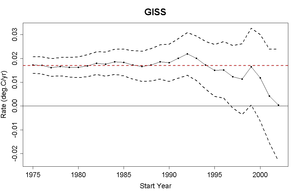
Let’s consider the trend up to the present (through June 2011) from all possible starting years 1975 through 2002. I’ll use GISS monthly temperature data, and I’ll treat the noise as ARMA(1,1) noise when estimating the uncertainty in the trend. That will enable me to compute what’s called a “95% confidence interval,†which is the range in which we expect the true trend to be, with about 95% probability.
To show PeteB what we get using data I did this for a start years from Jan 1975 through Jan 2002:
Took the GISTemp time series from January of the start year through August 2012. Used “arima” in R to obtain the best trend under the assumption that the data consisted of a linear trend + ARMA(1,1) ‘noise’. Plotted the best trend with black circles and the trend ± the arima estimate for the 2σ uncertainty in the trend.
The trend and the estimated uncertainty intervals obtained are shown below:

(Update:I couldn’t help myself. I added to the graph. 1:43 pm.)
I added a trace to indicate the nominal value of 0.2C/dec projected by the IPCC. That nominal trend is close to what one gets for the multi-model mean computed either from 1980-to now or 2000-now. I have omitted a 0 C/dec trace and also omitted Tamino’s red trace at 0.17C/dec trace. I’m sure a number of people will use the eyeball method to figure out where it is … or just run the script. (Link provided below.)
I’m not certain I did exactly what Tamino did. But this is what I get if I do what his text appears to explain. (He’s done somewhat different -shall we call them “tweaks”?- in the past. But I’ll refrain from commenting on those unless he repeated them in the post commenting on Goddard.)
I’d also note: I suspect if I were to run Monte Carlo cases for ARIMA(1,0,1) cases this method slightly under-estimates the uncertainty intervals. Note that I am not using this method in my comparison post. the uncertainty intervals I have been showing are nearly always wider than those computed using ARMA(1,0,1). But I’m under the impression the method itself is standard enough provided one is confident the ‘noise’ is ARMA11.
Here’s the R script: Taminos_Goddard_ARMA11
Update:Arthur Smith asked why I didn’t end in 2003 when recreating Tamino’s graph that ended in 2002. Ending in 2003 would make the final trend almost 10 years long which is as long as the final trend on Tamino’s graph was when he created it in 2011. Here is with the final trend computed starting in 2003:

What we now see is:
- The final 3 points show the observed trend inconsistent with warming at a rate of 0.2C/decade. In my previous graphs only the final 2 points show that. So adding this third point makes the model’s ability to forecast look worse that it looked without the extra point on the graph.
- The final two points show a computed best fit trend that is negative. Previously only one point showed a negative trend. So, adding the 10 year trend shows that the choice of 2002 may not be quite as bad a cherry pick as Tamino suggested. (I do think it was a cherry pick to some extent– but you get a negative trend with 2003 too.)
Update Nov. 26 Arthur wants to discuss trends up to starting in 2008.

BTW: I can’t help but chuckle at this
The upper open circles sure do dip below the horizontal dashed red line now!
May I ask if this his a true statement, statistically speaking
“There has been no significantly significant upward trend in the past 10 years”
As to me it looks like 2002 is zero.
DocMartyn, significant^2 ?
Doc–
If we use ARMA 1,1, if you limit trend computations periods starting in January and use GISTemp, then you can say that there has been no statistically significant upward trend since 1995. You determine “statistically significant warming” by comparing the lower circles to the dashed line indicating ‘0C/d’. Warming is statistically significant when the lower circles are above 0C/dec.
Bear in mind: I don’t think “no statistically significant warming” means much. It’s a “fail to reject” statement. “Fail to reject” will always happen if the time period is sufficiently short.
(The difficulty is that those defending models want to turn this upside down and complain that we shouldn’t take “Reject” seriously because of short time periods. That’s not right. If we get a ‘reject– as we are for 0.2C/decade right now, the “too short time period” is not a valid criticism. Valid criticism exist but that one is not one of them.)
I know Tamino stopped at 2002 – but that was over a year ago. Why did you stop at 2002?
Arthur– PeteB asked me to compare what I got to what Tamino did so I used the years Tamino used to make the comparison. That’s pretty much it. Pete B did want to know how things changed for a start year of 2000 specifically. I’d been showing that in the previous post. Had Tamino’s post not included that I would have added that to address his question. But — basically PeteB wanted to know how that specific graph of Tamino’s would change with the addition of another years data and that’s what I showed.
I assume Tamino ended in 2002 because that’s the start year Goddard used in his post. So that seems to be the original basis for ending the analysis in 2002 and it seems to be given the narrative about commenting on Goddard’s choice, that’s an appropriate choice.
notes the arrival of a climate attack blogger – someone who reviewed Mann’s book before it was published
diogenens–
Who reviewed what book and your suspicions of when they might have reviewed it are not relevant to this post.
you are right, Lucia but it is still interesting to check the arrivals of the “attack dogs”. I smile when I note that a book that was published on March 6, 2012, was reviewed by Stephan Lewandowsky on January 29 and by Arthur P Smith on February 1.
diogenes– Arthur has been commenting here since 2008. Also, your analysis is overlooking the possibility that Arthur was sent a copy by the author prior to official publication. That happens. It’s not even uncommon.
I would imagine that if Arthur received an advance copy that he would indicate this in his review as required by Amazon rules.
lucia, I think you misinterpreted diogenes’s point. My impression wasn’t that he is “overlooking [that] possibility,” but rather, making a point based on it. Copies of MIchael Mann’s book were distributed early to a number of individuals to get a bunch of glowing reviews right off the back. It was a PR move (coordinated in part by John Cook). Someone being involved in a move like that could be taken to indicate things about them.
In the same way, Arthur Smith may have been commenting here for years, but he doesn’t comment on that many posts. The fact he posted on this one, one sort of critical of Tamino, within hours of it being posted, could be taken to indicate things about him.
Or at least, that’s how I interpreted diogenes’s remark.
To add to Steven Mosher’s remark, Amazon’s rules for reviews say:
There are a number of reviews posted to Amazon from people given a free copy specifically so they’d write good reviews. To my knowledge, not a one disclosed that they had received a free copy, much less that they were given a free copy so they’d write a positive review.
diogenese,
Early copies of a book (or even journal article) almost always will be sent to those expected to give glowing reviews. Mann sure wasn’t going to send Steve McIntyre an early copy of his book. 🙂
.
Like lots of people, Arthur Smith seems to comment selectively on subjects which interest him. The general category in this case is ‘any post which suggests or implies low climate sensitivity’. ‘Attack dog’ seems more than a bit unfair.
SteveF, if all one was going off of is what topics Arthur Smith finds worth discussing, I’d agree it’d be unfair to consider him an “attack dog.” However, he is an active participant in the “blogosphere,” so there is a lot of material to draw from.
I won’t go into details as I don’t think anyone wants that, but my experience with him is he doesn’t post enough to be considered an “attack dog,” but otherwise, the description fits well. I have seen him make many unsubstantiated attacks against people, often based upon what appear to be misrepresentations and/or willful delusions.
Coordinated attack dogs or not, if they ask a good question then why not? If they start posting links that SkepticalScience pseudo-science then its time to complain.
Brandon– Maybe I misunderstood. But I don’t want this thread to be a discussion of reviews of Mann’s book at Amazon.com or whether people might or might not be “attack dogs”. Arthur’s question was on topic.
Fair enough.
So i’m just curious – how many of the models have correct aerosol forcing values for the 2000s or are they just set to zero (or assuming a decrease rather than increase)? It’s a fun game to play where we all look at the multi-model means and use the CIs to determine the accuracy but somehow I get the feeling that all models are not created equal…
thanks lucia – very interesting looks like we are getting to the point where the reduction in warming trend is becoming statistically significant
Lucia, what trend would be required whereby one could reasonably state that there has been no statistically significant warming for 17 years?
I only ask because Ben Santer said he’d become a sceptic if that happened (note: I may have exaggerated this a bit). 🙂
cui–
Do you have a quote? Did he say no statistically significant warming? Or that he’d be a skeptic if the trend wasn’t above 0?
Also– which noise model? In his paper on tropospheric trends he used AR1. That makes narrower uncertainty intervals. Consistency being what it is….. those seem to be “allowed” if one is proving warming, but “not allowed” if one is showing models are off. (Because using that, the models are waaaaayyyyy off and have been consistently for some time now.)
I have good guess on what Tamino did, I am close to replicating his graph, take a look:

http://i46.tinypic.com/1ovbbq.jpg
I have limited the data to 1975 to June 2011 to match the same data as Tamino. I calculate the trends from January every start year to June 2011. To estimate the arma(1,1) uncertainty intervals I use the method outlined by Tamino ins his “Alphabet soup part3a + 3b” and “Hurst” posts. I estimate the arma parameters over the whole period 1975-2011, and then use Neff = N/v, where v= 1+2*rho[1]/(1-phi), rho[1] is lag 1 autocorrelation and phi is the AR coefficient. Replacing N with Neff can then be obtained by multiplying the OLS errors with sqrt(v). Check the code from Foster&Rahmstorf to see this implemented.
With this approach one cannot reject the AR4 projections.
SRJ–
I thought he might have done that.
If so, his results rely on cherry picking a data to create a “noise model” with in appropriately wide uncertainty intervals. That is: He is specifically picking a period when major volcanoes erupted. During that period, the models themselves say the mean (not noise) is non-linear.
But his method treats deviations from linear by the mean as noise and throws that into his estimate of the noise and it’s correlogram. The consequence of this is to widen error bars above the level that is appropriate if you goal is to estimate the variability of trends over repeat samples of the same period.
This matters because what those uncertainty intervals are supposed to be is an estimate of the variability of trends over repeat samples of periods with similar forcing. They are not– for examples– supposed to be an estimate of the range of trends we might have gotten had Pinatubo or some other volcano had a stratospheric eruption at some time between 2000-now.
The general principle that you should only include “the noise” when estimating the properties of “the noise” must be well understood in statistics. It is well understood in other fields where statistics is used and applied.
But anyway: If tamino’s error bars are what you say they are, then his decribe the amount of variability that one estimate if we were forced to pretend we had no idea whether volcanic eruptions went off when they did and/or had no idea that those eruptions do affect the temperature trends. In such a case, the variability due to Pinatobu, El Chicho etc. would by a mistery to use and we would have to decide that “for all we know” the “same” thing could have happened during any period at the same rate it happened during the full 1975-now period.
But… in reality, we know the volcanic eruptions have a major effect and we know when they went off. So computing the uncertainty intervals during periods when we know these major eruptions did not occur using uncertainty intervals based on the assumption that we have no idea whether they occurred or not is called “cheating”. Fishing out a time period where one knows the occurred to estimate “universal” estimates of the time series properties is called “cherry picking”. If Tamino did as you said, he did both.
My bad, I think, but I’d appreciate your comments.
He was talking about lower troposphere (TLT).
“Because of the pronounced effect of interannual noise on decadal trends, a multi-model ensemble of anthropogenically-forced simulations displays many 10-year periods with little warming. A single decade of observational TLT data is therefore inadequate for identifying a slowly evolving anthropogenic warming signal. Our results show that temperature records of at least 17 years in length are required for identifying human effects on global-mean tropospheric temperature.”
I’ll even link to the fount of all wisdom:
http://www.skepticalscience.com/print.php?n=1333
cui–
In that paper, Santer used AR1. That will give tighter error bars– and we would reject the multi-model mean for surface temperature using those and would have at the time that paper was published. Those testing models then seem to have “discovered” the inadequacy of AR1. Nevertheless, I’m sure that if one shows that the trend is not statistically singificant using the wider ARMA11 error bars, he would just say you should use the tighter AR1 ones– for testing the “no warming” model. (But they would remain inadequate for saying the models are off. 🙂 )
(Yes. I am being snide. But collectively, this is happening.)
Lucia,
“cheating” “cherry picking”
” If Tamino did as you said, he did both.”
Now why would a smart guy like Grant do that? Perhaps there is a desperate, viseral need to not admit the models are running too warm. I am not being snide. 🙂
Lucia,
I do not understand your point. And I am not even sure you understood my approach.
To clarify, here is another plot.
In blue I have plotted the same uncertainty intervals as before. These are calculated with arma(1,1) parameters estimated over the period 1975-2011. E.g. for the data point in 1999 the trend is calculated from January 1999 to June 2011, while the arma-parameters are estimated over January 1975-2011.
The reason to do this is that Tamino explains that you need lots of data for estimating the arma parameters reliably.
In green I have plotted uncertainty intervals calculated with arma-parameters estimated over the same periods as the trend. E.g. for the data point in 1999 the trend is calculated from January 1999 to June 2011, as are the arma-parameters.
http://i47.tinypic.com/1zvwrwz.jpg

Besides that, Tamino does not compare the trend estimates from that graph with the climate models. He is only comparing trend estimates over different periods of time to see whether they are significantly different from the long term trend since 1975.
The word climate model is not mentioned in his post. It was PeteB and you that started comparing with climate models.
Tamino’s approach is purely statistical and could be applied to any time series with the same statistical properties, regardless of the data being temperature or no. of potatoes eaten pr. year.
I think your accusation of Tamino doing cherry picking is wrong in this case.
Steve F,
Tamino was not comparing these trends with climate models
I thought we had established that volcanoes had minimal impact, especially compared to ENSO?
.
The way I see it, *your* method consists in faulting the model for failing to capture middle-term fluctuations (like ENSO) which the ARIMA fit (on monthly data!) cannot “see”.
.
The problem with this is that the models don’t claim to be able to capture these fluctuations in the first place.
Hehe! Thanks Lucia. You’re always entertaining and certainly right. 🙂
@SteveF: “Smart Guy Grant” extrapolated linear interpolation of a time series for decades in the conclusion of his recent paper. That’s the kind of mistake that new users of Excel (“Hey, Apple’s up 10% today, so if I wait for a month, it’ll be up 1700%!”) make. I think he’s very smart, but suffering from a severe case of confirmation bias.
SRJ (Comment #104009)
You repeat here:
What I am saying is given our knowledge of what happened with volcanic eruptions during the period from 1975-2011 and and what happened during the period from 1999-2001, computing the arma parameters using data from 1975-2011 and usign them to compute uncertainty intervals for trends for the period from 1999-2001 is both cherry picking and cheating. That is: I am saying the uncertainty intervals computed the way you computed the blue ones is “cheating” and “cherry picking”.
Have I understood what you did correctly?
I never said he compares them to climate models. In a comment I pointed out that he does not compare them to climate models. In fact– I’ve noticed that he has gone utterly silent on this topic. 🙂
So? People are allowed to discuss other features. Goddard didn’t mention trends from 1975, but when discussing Goddards post about trends since 1975, tamino added trends from other years.
Then show it. The fact is: It is well accepted that volcanic eruptions cause ‘dips’ with subsequent recoveries in temperature series. It is well accepted this is a deterministic effect. I only mention models to show an example where this is reflected– but the principle is well understood. Moreover, Tamino knows it because he includes volcanic aerosols in some of his multiple regressions.
So: Tamino knows that an important effect:
1) Volcanic aerosols would result in high deviations from the linear trend during the period from 1975-2011.
2) That such deviations would not occur during the period from 1999-now.
3) That the character of the ‘noise’ would be affected by this.
4) That if you estimate the character of the “noise” using the period with volcanic eruptions, that “noise” will have a) higher standard deviations from the mean and b) higher auto-correlations and result in higher estimates of the ‘variability of trends’ for repeat samples.
5) He either knows– or ought to know– that the estimates using ARMA are supposed to be estimates of the variability of repeat samples over the same time periods with similar forcings. They are not supposed to be estimates over repeat samples were possibly a volcano might have gone off in 2001 (etc.) but we just don’t know.
So, he either knows or ought to know that computing the ARMA11 parameters to describe uncertainty as if we don’t know that volcanic eruptions went off and applying them to a period in which we know they did not go off is incorrect. Since he either knows or ought to know that this method results in higher uncertainty intervals that one would get if these were estimated fairly and he gets an answer he seems to “like” better than he would otherwise, what he is doing is both a) cheating and b) cherry picking.
If you think what he did is not cheating or cherry picking you are going to have to explain why it is ok to compute the ARMA parameters using data from 1975-2011 knowing volcanic eruptions were rife during that period and then applying them to the period from 1999-2011 knowing that no volcanic eruptions occurred during that period.
SRJ
I want to comment on this:
Yes. And using your analogy I still conclude his method is wrong. It would be wrong to estimate the variability in potatoes eaten during years when we know crops did not fail basing the estimate of variability using a period that included years when crops failed repeatedly (e.g. Irish Potato Famine). Moreover, if he knew that the “crop failure” factor differed in the period when he estimated variability and nevertheless applied it during the period when it did not, and doing so got him an “answer he liked better”, this would be classic cheating and cherry picking.
@SRJ: Let me try to explain, perhaps from a slightly different angle.
There’s a tradeoff between a model being more useful and a model being more falsifiable. Huge error bars are generally a bad thing, since they make a model less useful (even less credible, perhaps), but they do make it less falsifiable. Predict a huge range of things and you’ll probably be correct, though no one will really care.
So, in general, we don’t want to lump lots of things into the catch-all “noise” category, we want to pull out things that we can model and model them, decreasing the noise.
For example, I was once modeling electricity usage for an organization and my first, naive cut at it resulted in forecasts with +/- 50%. Try presenting that to someone working on a budget! So I dug in deeper and found several things I could model and finally got the forecast interval to less than +/- 10%, which was useful.
In Tamino’s case, his incentive is for the opposite: enlarge the error bars to make the model less falsifiable. And I think that’s what Lucia’s getting at: he’s not pulled out known effects, but is leaving them in the “noise” category to increase his error bars. (Which is the only thing saving him at the moment, since the point estimates look very unfavorable.)
You tried to address this by using shorter ranges of data, but you didn’t actually change the components or characteristics of the “noise”. (In fact, as you noticed, you made things worse since your parameter estimates’ CI’s probably exploded as you decreased your data length, so your second set of error bars was increasingly nonsensical.)
So the appropriate next step is to dig into the data and pull appropriate things out of the “noise” category and into the “modeled” category. Perhaps there is nothing to pull out and it really is all noise. Lucia disagrees.
If I understand the argument.
Wayne– It’s worth nothing that Tamino himself explains part of the deviations using metrics that capture the volcanic effect. If he consistently denied that volcanic eruptions do cause deviations, I would not consider this “cherry picking” or “cheating”. I would just disagree with his view on whether or not volcanic eruptions can cause temperatures to dip and then rise again.
But I know that Tamino– like pretty much everyone else including modelers– does ascribe dips and recoveries to Pinatubo. He does not dispute that the multi-model mean is correct to show these dips after eruptions that are sufficiently violent to throw stuff into the stratosphere. In fact, other posts indicate that he seems to agree this should be so.
Despite that he periodically resorts to ignoring this when computing uncertainty intervals in those posts where it would suit his narrative to have wider uncertainty intervals.
That’s why I call “cheating” and “cherry picking” rather than just a mere disagreement over what volcanic eruptions do.
SRJ (Comment #104009),
No, Tamino did not compare to the multi-model mean. But it seems to me reasonable to see if Grant’s analysis is a) correct (it is not) and b) if his analysis approach, when done correctly, has implications for the statistical validity of the AR4 climate model projections (it does, the models are running warm). Do you not find this interesting?
Wayne2,
“I think he’s very smart, but suffering from a severe case of confirmation bias.”
Of course, just as most climate scientists seem to, especially the “stars” in the field.
.
Which is not to say the same does not happen in other fields (it does!). But the large public policy consequences and potential societal costs make confirmation bias in climate science less acceptable than in any other field, including drug trials, where despite explicit and widespread efforts to reduce bias, it’s influence is obvious. In climate science there doesn’t appear to be even a halfhearted effort to reduce confirmation bias. It is a sad commentary on the maturity of the field: importance similar to nuclear weapons, conducted like it were ‘trendy’ research in psychology.
I did not receive an advance copy of Mann’s book; I purchased and reviewed the Kindle edition which was released January 24th, as can be seen on the Amazon page:
http://www.amazon.com/Hockey-Stick-Climate-Wars-ebook/dp/B0072N4U6S
and you will notice that my review is labeled with:
“Amazon Verified Purchase” which proves that I purchased the book *before* I reviewed it.
I would note that diogenes’s accusation above is a perfect exemplar of the conspiracy ideation which Stefan Lewandowsky has been investigating. I do appreciate Lucia somewhat standing up for me as not being an “attack dog”, but nobody seems to have taken the simple step to discover that diogenes claim was completely unfounded – so much for “skepticism”. Thanks for another datapoint diogenes!
Lucia,
your interpretation of my approach is correct.
“If you think what he did is not cheating or cherry picking you are going to have to explain why it is ok to compute the ARMA parameters using data from 1975-2011 knowing volcanic eruptions were rife during that period and then applying them to the period from 1999-2011 knowing that no volcanic eruptions occurred during that period.”
Because the graphs is produced as a response to people claiming things about trends with different start periods.
Tamino shows what happens if you start you calculation in different years. It is just a simple statistical exercise, not considering of the underlying physics or data generating process (though I hate that word).
If I understand Taminos points right, he would also argue that using data only from 1999-2011 gives too uncertain arma-parameters.
In any case, I do not think that he is cherry picking. My impression is that he used that used data from 1975-2011 to make sure that his estimates of the arma-parameters were reliable enough, implicitly assuming that the arma(1,1) model is valid over the whole period.
Well, I think we will have to agree to disagree on this matter about Tamino cherrypicking or not. I think he had valid reasons for the choices he made about the data used for calculating uncertainty intervals, you disagree.
I do see your point about volcanoes affecting the noise variability. We can loosen up the restriction about having lots of data and then calculate the arma-parameters over the same years as the trend. I.e. we are trading off some reliability in the parameter estimates but then we are taking into account the changing properties of the noise, due to e.g. volcanoes.
I showed the result of that in my previous comment.
Taminos point was that no trends are significantly different from the trend since 1975, and that still holds true using my modified approach (green lines). Using your approach with arima(1,0,1) the last three trends are different from the long term trend since 1975.
I agree that you can do more complicated things to estimate the uncertainty, the approach from Taminos graph is just a first quick estimate, at least that is how I think it should be considered.
I will be curious to see how you guys would do this in a more rigorous way that could deal properly with volcanoes.
Lucia, I have not been following these threads closely but in looking at Tamino’s R code I find he is using the sd of trends, whereas, as I recall, in earlier threads you talk about using the se of the trends. Here is the function he develops for obtaining the regression trend slope and the sd of the slope for evidently ever shortened periods of time coming forward. It is almost like the difference one might expect using confidence interval limits versus limits from prediction intervals for a trend. I just had a percursory look so I might be mistaken in what I see.
ms_and_sms<-function(temperatures,year=1975){
norm_months=c(1:length(temperatures))-mean(c(1:length(temperatures)) )
fit=arima(temperatures, order = c(1,0,1), xreg=norm_months, include.mean=TRUE )
var_m=fit$var.coef[4,4]
m=as.numeric(coef(fit)[4])
return(list(m=m,sm=sqrt(var_m),year=year,n=length(temperatures) ))
}
I am in the process of using Monte Carlo simulations with Arima models to estimate CIs for the observed results of a GHCN segment and comparing those results with the more commonly used methods.
Back to the topic of this post – I actually downloaded Lucia’s R code (thanks Lucia!) and extended the plot to 2008. Interestingly, it’s only a brief period (2001-2005) that “rejects” in this way. 2007 is wildly in the other direction. It’s a nice way to show that things bounce around a lot, but I’m not sure it tells us anything (either what Lucia or Tamino were trying to communicate).
Arthur Smith:
I’m kind of there with you. As toto points out short-period climate noise is dominated by ENSOs, which are highly variable, as AFAIK unpredictable, and this variability is poorly if at all captured by climate models (see e.g. the AR4 summary, if I’m reading it right, their ENSO amplitudes are almost uniformly too small by a factor of 10 in amplitude.)
I understand that Lucia was just redoing what tamino had already done, only maybe more correctly, so this really is addressing the underlying premises put forward by tamino, who dreamed up the exercise to start with.
Anyway, IMO the underlying problem is that the ensemble of climate models are not capable of producing realistic climate noise over these time periods, so you’d have to adjust the models for this additional noise—which the models aren’t yet up to being able to predict—if you really wanted to statistically compare observed to modeled trends.
Put it another way, IMO, the apparent failure of the models to validate is really the failure to produce realistic ENSO patterns, and that is thought to be substantially a resolution issue (granularity of the models).
It’s not a failure of the physics of the models if a realistic solution requires a bigger computer than they can currently fit their models into (unless there were another method that allowed a more compact representation and a more efficient solution, but that doesn’t seem to be in the cards).
SRJ
Huh? The graph was produced in an article commenting to Goddard’s post writing something about a trend since 2002. Goddard didn’t say anything at all about different start periods.
Tamino added what he wanted to add to make points Tamino wanted to make. That’s pretty standard. But people get to observe, criticize of comment on Tamino’s cherry picking. The could do so even if all Tamino had been doing was commenting on people claiming things about trends with different start periods!
And in doing show, he elected to show uncertainty intervals which are computed using a flawed method. And his discussion goes on and on about what we learn from the magnitude of the uncertainty intervals.
If he didn’t cherry pick periods to compute his uncertainty intervals he would have showns the green ones– not the wider blue ones. My cherry pick statement applies to his decision to use a method that showed the blue uncertainty intervals. That’s it.
Goddard showing the trend since 2002 was also a “just a simple statistical exercise, not considering of the underlying physics or data generating process”– and Tamino criticized his choice as cherry picking. The fact is: being “just a simple statistical exercise” does not preclude cherry picking. Of if it does preclude it, you have to decide that Goddard did not cherry pick by using 2002 as a start year.
This is a claim Tamino makes. As with most cherry picks, it is covered with a plausible excuse. (For example: Goddard’s cherry pick is justified as being a 10 year trend- which is a round number. Tamino criticizes Goddard for this. But it is true that 10 years is a round number and it is true that people often report 10 year trends precisely because they are round numbers.)
On the truth part in Tamino’s claime: Using a short data periods does give uncertain data parameters. This is true for all statistical analyses.
But the correct way to fix the problem of possibly too small error bars due to a short period is to run monte-carlo to estimate the effect and fix it (if it exists). Finding a period with uncharacteristically high variance due to volcanic activity is not the correct way. It’s cherry picking and remain so even if one can can concoct a ‘cover story’ like “Ten is a good round number” or “I wanted a lnger period of time.”
If estimating since 1975 is somehow better than estimating since 2000, why not estimate the uncertainty intervals using data since 1900? Surely if 36 years gives less uncertainty in our knowledge of the ARMA parameters, using 112 would do an even better job, right? Why not pick that period? These are real questions and they cut to the issue: Why start in 1975 to “freeze” your ARIMA model? I would suggest you do this exercise bearing in mind that all the data are known to the analyst before he or she selects 1975 as the start year.
If you mean we could use the green trace. Sure: We could. Had Tamino used the green trace, I wouldn’t say he cherry picked. I would merely say he got a graph based on data that ended in June 2011– which would have been fine. But of course we’d update as we got more data.
I don’t disagree that Tamino could have said substantially the same thing back in july 2011 withouth cherry pickig his uncertainty intervals. I merely pointed out that — among other things– he did cherry pick them. He did: He showed teh blue cherry picked ones rather than the green ones.
Moreover, if you look at the green ones in your graph, had he shown the green trace, we would see that using a start year of 2002, the IPCC projects were now outside the ±95% confidence intervals of consistency with observations. Note your greent race falls below 0.2 for the final point.
Because the nothing in the 20th century can possibly be considered a test of forecasting ability, the green trace falling below 0.2 C/decade after 2000 has important implications with respect to diagnosing any possible bias in the multi-model mean for climate models. Even if Tamino elected to not show the IPCC trend of 0.2 c/dec and even if he didn’t discuss where that trend fell relative to his computed uncertainty intervals, I have very good reasons to believe that Tamino would not have wished to show that green trace falling below the dashed red line on any graph he creates. Ever .
As I said: I would not have criticized Tamino for cherry picking if he’d used the green trace. It’s acceptable.
Sure.
But that’s a pretty big subject change relative to anything I wrote about in my post. My post is a response to a question from PeteB. PeteB wanted to know why my uncertainty intervals were smaller than the ones in Tamino’s post.
Was it because of the extra year of data? (Yes. In part) Was it the method? (Yes. In part– Tamino used a non-standard method that permits him to cherry pick to find periods with different sized intervals. He picked ones that result in smaller intervals– tha tis he gets your wider blue ones rather than the green ones.)
I engaged PeteB’s questoin and gave him his answer to his question. This is permitted even if Tamino was discussing something else. And Tamino was cherry picking to get wider uncertainty intervals even if he wasn’t testing models.
If it’s quick– why don’t you make a graph using data through August 2012. It would be interesting to see Tamino’s graph updated using your blue and green bands. I bet PeteB would like to see it too.
Lucia – Tamino certainly uses volcanic aerosols as suits him. The effect of Pinatubo was prominent in the Foster-Rahmstorf paper arguing that Hansen had got all of his predictions spot on.
From their abstract: “When the data are adjusted to remove the estimated impact of known factors on short-term temperature variations (El Niño/southern oscillation, volcanic aerosols and solar variability), the global warming signal becomes even more evident as noise is reduced.”
Meanwhile, if the trendline has error bars which equate to +2.5C to -1C per century, we should perhaps remain calm. 🙂
Arthur Smith (Comment #104027)
Can you post a plot of the results?
Arthur
It only rejects in the period where one might test forecasts: That is, in the 21st century. The models aren’t so bad if they are testing using data available for tuning while they were ‘built’.
Everyone agrees that “fail to reject” over short periods doesn’t mean much. I’ll post the graph in a second. I’m not sure what you mean by wildly the other way” in the final year. What I see is the uncertainty intervals grow and for short period of times we “fail to reject” both the hypothesis that m=0 C/dec and m=0.2 C/dec. Fail to reject at very short intervals is not– by any stretch of the imagination- a contraction of “reject” at longer intervals. I think you understand this when people are crowing about Phil Jones admitting that we have “no statistical warming since 19??”
Carrick (Comment #104029),
 While this is only for ocean areas, what jumps out (for me) is how clear the volcanic influence becomes and how much reduced the the overall variability is… and even more so if you were to subtract some reasonable estimate for the volcanic effects; the whole trend would be pretty smooth, with a fairly steady rise from 1979 to 2001, and flat to slightly falling post 2001. The other interesting thing (off topic) is the appearance of “tropospheric amplification” short term, but its complete absence long term.
“so you’d have to adjust the models for this additional noise—which the models aren’t yet up to being able to predict—if you really wanted to statistically compare observed to modeled trends.”
.
Or adjust measured temperature trends to account for the influence of ENSO sort of like this:http://i45.tinypic.com/166g7bc.png .
@SteveF: The more I think about it, the more I believe Tamino is very good and thorough with the math. He’s just not very good at the deeper issues of making reasonable hypotheses, models, etc.
Like I said, I looked at F&R 2011 and couldn’t believe the final two sentences: “This is the true global warming signal. // Its unabated increase is powerful evidence that we can expect further increase in the next few decades, emphasizing the urgency of confronting the human influence on climate.” Essentially projecting a straight line for “a few decades” off the end of his data.
In that paper, he lumped everything other than the three natural forcings they were considering into a catch-all “global warming” category, which obviously maximized that. Now, he juggles things around and lumps the same natural forcings into “noise”, when it suits him, as Lucia points out.
(The example I gave earlier about electricity forecasting was a real eye-opener to me. I knew that I was lumping all kinds of things I didn’t want to worry about into “noise”, but didn’t realize how worthless it would make my forecasts. I had one of those heart-in-your-throat moments when I imagined telling people, “I project you’ll spend $200,000 next year for electricity… plus-or-minus $100,000.”)
SteveF, if your point is to use 30-year trends, that is one I can endorse. I don’t think any of the people calling for immediate action are going to be very happy about it though.
(I know yo know this—using smoothed data is visually useful for humans, but unless you are doing non-linear processing, there isn’t any advantage in terms of trend uncertainty in presmoothing the data.)
It is striking how much less noisy the oceans are than the land surface air temperature. You kind of expect this when making measurements in the surface boundary layer, which is stirred up by convection and weather, but … to me still striking.
To followup on that comment, you can’t use a 20-year period of overlap between model and data to validate the model, if the data were present when the model was written (Lucia’s point to I think).
You really need 30 years of solid data, 20 is an absolutely minimum. I had done this trend uncertainty using a Monte Carlo based approach and assuming homoscedasticity (this is a best case assumption, if Hansen is right, that means the variability is increasing over time, and the period you need to use to resolve 0.2°C/decade just gets longer). The 95% CL from one of Lucia’s posts are shown for comparison.
I don’t recall the particulars of how she obtained those estimates or whether they differ from the ones shown here, but it’s clear she’s not understating the uncertainty in her analyses.
Carrick,
Smoothed data (11 month centered average) is for human consumption only, and has no influence on trend uncertainty. 😉
.
My point was that adjusting raw measurement data by removing known (identified) short term influences like ENSO and volcanoes reduces variability, and helps to reduce uncertainty in the underlying secular trend. As to whether or not 30 years is better than some other period: I guess it depends on the data itself. In my graph there sure looks to be a change in the trend near 2000; whether or not that is statistically significant can be tested, but the chance of finding a significant trend is improved if known sources of short term variation are first removed from the data.
.
If there is a pseudo-oscillation with a period of ~60 years and an amplitude of ~+/-0.1C, superimposed on a GHG forced trend, as many have suggested, then looking at a 30 year period (say 1970 to 2000) could give an exaggerated estimate of the response to forcing, while 2000 to 2030 might give an underestimate of the response to forcing (as I am sure you are aware).
Wayne2, X +/-50%X is a quite reasonable range in many things.
Have a go at how much will be spent on my healthcare next year; nice error bars.
Official US inflation figures now exclude anything most folks might actually buy (food, fuel…), I believe. So it’s like 2-3%?
There is a samizdat inflation figure based on what used to be included. It’s strangely different. 10%+.
Just saying, if we’re excluding things….
SteveF:
OK I wasn’t sure that’s what you were talking about. Of course if you have an additional explanatory variable, I agree it helps to remove it.
Example: I’m characterizing a sensor at the moment that is grossly sensitive to temperature. I also expect it to be sensitive to atmospheric pressure (physics based reasons why it has to be), but if you don’t cofit for temperature and atmospheric pressure (or first subtract off the temperature dependence), good luck extracting out the % effect of e.g., a 1kPa increase in atmospheric pressure.
@Carrick (Comment #104039): You say “if Hansen is right, that means the variability is increasing over time”. Do you mean his recent paper (nicknamed “Loaded Dice”)?
I’ve actually been walking through that paper/data and as far as I can tell, he only proves that if the mean in era B is greater than the mean in era A, maximum values in era B will tend to be farther from era A’s mean than maximum values in era A are. That’s so blindingly obvious that it’s easy to misunderstand and think he’s talking about variability in era B versus variability in era A, but he’s not.
(Not to mention that era A ended and era B began in 1980, so isn’t very applicable to the current discussion which begins in the 1990’s.)
Or were you talking about another Hansen paper?
Lucia
(thanks for fixing my graphs so they show up in the comment)
“If it’s quick– why don’t you make a graph using data through August 2012. It would be interesting to see Tamino’s graph updated using your blue and green bands. I bet PeteB would like to see it too.”
Sure, no problem. I have also added the estimates from the arima-function, dashed red is trend estimate, thick red is 95% CI. To make comparison with my earlier plots easier the last trend showns is from 2003-2012, as before.

http://i45.tinypic.com/2j4t086.png
14 more months data do make CI’s smaller, so that the upper CI for the long term trend since 1975 now is just above 0.02 for the approaches using OLS and adjusting via the arma parameters. The CI’s for the long term trend from arima(1,0,1) do not include 0.02.
“If estimating since 1975 is somehow better than estimating since 2000, why not estimate the uncertainty intervals using data since 1900? Surely if 36 years gives less uncertainty in our knowledge of the ARMA parameters, using 112 would do an even better job, right? ”
My answer: Because since 1900 you cannot model the temperature as a simple linear trend + noise. There is a breakpoint in the temperature series somewhere around 1970 plus minus 5 years, depending on the method you use to estimate the breakpoint.
So to keep it simple, one starts in 1975, after the breakpoint.
I guess one could fit a piecewise linear model and then estimate the arma-parameters for the residuals from that model.
” if Hansen is right, that means the variability is increasing over time, and the period you need to use to resolve 0.2°C/decade just gets longer). The 95% CL from one of Lucia’s posts are shown for comparison.”
Well, its largely a methodological artifact. stay tuned.
@SRJ: Thanks for you graphs, etc! I’d note that in the best case (blue line), Tamino is vindicated, but in the other two cases he is not. But even in the best case, the lower bound for starting years of 1997 and later includes zero. Seems to me that’s a problem in and of itself.
Hi Lucia – I have a comment (#104023) in moderation regarding diogenes’s attack on me in this thread – since his comment contained a provably false statement I hope you will either approve my comment or snip the entire discussion. Thanks.
I don’t know how the IPCC projections could have predicted the observed global temperature numbers much closer than what we have seen. All these statistical machinations trying to challenge AR4 are silly as there simply is not enough data to say anything useful about the success of their projected temperature trends.
–
On the other hand there is starting to be enough history to get some ideas about the validity of AR3 projections. Those projections, based on models run in the late 1990s, now have around 8 years of post-dictions and 14 years of predictions to check against observations. UAH, for example, shows a 0.17C/decade LT warming since 1990 vs the AR3 predicted 0.18C/decade.
http://s161.photobucket.com/albums/t231/Occam_bucket/?action=view¤t=fig9-15ahighlighted.gif

–
As to these graphs showing trends from different start dates, (which again include trends based on dubious amounts of history), they would show remarkable agreement with AR3 if they included the impact of the ENSO and solar insolence – as I have done below.
–
http://i161.photobucket.com/albums/t231/Occam_bucket/LTModelVsObsTrend.gif

–
–
PS.
Are there directions somewhere on how to insert a graphic in a post?
Arthur–It’s released from moderation. I didn’t realize it was there– it must have been there a while. Sorry I didn’t notice sooner.
Dave E–
The directions for inserting an image are:
1) insert a link to the image itself.
2) Wait for lucia to notice and add the html.
WordPress automatically strips html for images so you can’t do it yourself.
The Kindle edition of Mann’s The Hockey Stick Wars was published January 24 2012. Arthur’s review appeared February 1 2012. The review specifically states that Arthur read the Kindle edition, and the publication date thereof is easy to find. Diogenes’s (and some others) owes Arthur an apology.
I don’t know why you think this.
The third report was not called the AR3– it was called the “TAR” (T for third.) The second was SAR. The difficulty was that FAR would then be first, fourth, fifth and so on. So it’s the AR4. As for the projections in the TAR– that report predicted slower warming than the AR4. We are seeing less warming than in the AR4.
Wayne2,
” But even in the best case, the lower bound for starting years of 1997 and later includes zero. Seems to me that’s a problem in and of itself.”
This is often interpreted as meaning that you need to consider periods longer than 15 years, i.e. 1997-2012 to find significant trends. JeffId made a post in 2009 where he did this:
http://noconsensus.wordpress.com/2009/11/12/no-warming-for-fifteen-years/
Tamino have a similar post called “How long”.
In discussion of these kinds of graphs at SKS some statistically skilled person wrote that it is actually better to plot the statistical power of the t-test as function of the length of the trend period. Then you can see when the power becomes reaches some required level, and then you will know how many years of data you need to be able to detect a trend.
Btw. I think that linear trends are used way too much in climate discussions. It gives just too much discussions about when to start or end the calculation. I like the approach that Gavin Simpson is introducing here:
http://ucfagls.wordpress.com/2011/06/12/additive-modelling-and-the-hadcrut3v-global-mean-temperature-series/
Arthur–
You seem to think that not doing ‘research’ to clear you of whatever it was diogenese was accusing of you of indicates a lack of skepticism. I’m not going to spend time doing “research” to discover which books you’ve read or reviewed on Amazon, how you came to get the book, whether or not you followed Amazon rules etc merely because diogenese wants to come in and throw an OT stinkbomb to derail comments. My reasons for not doing it is that
a) I think discussions of who reviewed what at Amazon are boring and I don’t care.
b) I don’t want to waste my time pursing that issue because I don’t care about it.
c) I want to spend my time discussing the topic of this post and
d) I am perfectly content to wait for you to provide information available to you on this topic.
I suspect a number of other people neither believed of disbelieved digonese. And mostly, the thought that entire OT conversation was boring and not worth wasting any thought on.
I’m glad to see that you did read the book before reviewing. (I’d assumed that was diogenes complaint when I first read it. I never imagined he thought the possibility that you read it before the ‘official’ publication date was “the problem”. I guess I have now learned something (which I will make no effort to bother to remember.)
SRJ
Do you mean they did something like this:
http://rankexploits.com/musings/2008/falsifying-is-hard-to-do-%CE%B2-error-and-climate-change/
This is not quite right. Among other things, the power of a test is a function of
a) How far wrong the null hypothesis actually is.
b) and the confidence level you use to decree “statistical significance”.
c) the properties of your noise and
You never know (a), so when designing an study, you substitute a “detection threshold” to estimate the amount of data you will need to collect if the null you want to check is off by some specified amount.
So, for example, the AR4 has a nominal warming trend of ‘about 0.2C/decade’ and looking forward, we might estimate the variability to be what we saw in the past. ( Looking forward, we don’t know if volcanoes will erupt, so it’s fine to use those periods when predicting when you’ll see statistically significant warming. This estimate already includes the volcanic eruptions.)
Once you can do a calculation that tells you the probability you will reject the null of no warming (m=0C/decade) under the assumption that the actual magnitude of warmign is 0.2C/decade.
But what this does not tell you is “how many years of data you need to be able to detect a trend” . You actually need to specify the magnitude of the trend that you think exists.
But also: no matter what answer you get for your power, if you get a reject it’s a reject. The power estimate is only important if you have a fail to reject. In the graphs above, the model is telling us to reject the multi-model mean of 0.2C/decade. There is no “minimum number of years” for this finding to be meaningful because it’s not a fail to reject type finding.
Linear trends are used for testing the AR4 forecasts because the multi-model mean is nearly linear for the few decades of this century. So, while I have no objection to what Gavin did in that post– most of which applies to the hindcast not testing models– the fact is, if a forecast has a linear trend in its expected value, it’s fair to test that hypothesis by saying the individual realizations are “linear + noise”.
The Kindle edition of Mann’s The Hockey Stick Wars was published Jan 24. Arthur’s review appeared February 1. The review specifically states that Arthur read the Kindle edition, and the publication date thereof is easy to find. Diogenes’s (and some others) owes Arthur an apology.
Dave E.,
Please explain how you accounted for the influences of ENSO and TSI; without some explanation, the graphic does not mean much.
I wasn’t going to discuss the off-topic stuff again, but… there’s no way I can ignore this nonsense from Arthur Smith:
diogenes was wrong. Does that make his accusation “a perfect exemplar of the conspiracy ideation which Stefan Lewandowsky has been investigating”? Not at all. The coordinated PR move I referred to above is known to have happened. One can find undisputed information about it with a quick Google search.
Interestingly, Arthur Smith claims diogenes’s remark is “completely unfounded” because we can see he purchased a copy of Michael Mann’s book. However, he overlooks the fact purchasing a copy in no way prevents a person from having received an early copy.
In any event, I’m not sure “conspiracy” fits what was done, but if believing coordinated PR moves whose existence are public knowledge happened counts as “conspiracy ideation,” Lewandowsky’s work is even more rubbish than I thought.
Arthur:
Well in my case, and I suspect I speak for most everybody else who didn’t respond, I really just don’t care one way or the other.
Sorry I don’t find you and what you do particularly interesting. What you write here or other places I read, as it pertains to what I find interesting to contemplate or comment on, substantially more so. However, I didn’t seek out and read your review of Mann’s book, nor do I intend to, nor do I intend to read Mann’s book. Just not interested.
Never blame lack of skepticism when indifference will do as well. I figured if you wanted to defend yourself, you’d do so.
Sometimes I just shrug off criticism of myself rather than respond. You have the same freedom. There’s only so many daylight hours and I have other priorities that loom bigger than what somebody is saying about somebody on the internet.
Of course there’s a certain irony about Arthur making certain comments about Lucia on tamino’s blog (a place where she got banned for the temerity of noticing an error on the blog owner’s part), knowing full well she can’t respond to those comments on that blog. In fact these non-skeptics quite regularly engage in patting each other on the back in their little sport of kicking around people who don’t, can’t or are simply unaware they are the topic of somebody else’s criticism.
Arthur and Eli both probably want to skate softly on this point.
Carrick, I’m not sure what comments you’re referring to since I rarely visit that site, but according to a recent remark from Tamino, lucia isn’t banned for pointing out his mistake. He says:
😉
Brandon, I ran across that comment by accident.
Tamino can get very angry when you point out mistakes in his reasoning. I know that personally, and stopped going to his blog simply because if you can’t have reasoned discourse and you just have to take everything he says as gospel and smile, what’s the point?
Brandon Shollenberger
I guess historical accuracy is not his strong suit. He banned me after I pointed out that the two-box model he claimed we should have some sort of “extra” confidence in because it was somehow physically based violated the 2nd law of thermo. And I was right.
He did stop claiming we should have some sort of “extra” confidence in his model. This post is related to “the incident”.
http://rankexploits.com/musings/2009/two-box-models-the-2nd-law-of-thermodynamics/
“Please explain how you accounted for the influences of ENSO and TSI; without some explanation, the graphic does not mean much.”
——————————————————————————–
True. This is the basic formula I used for a predicted monthly global average temperature (assuming I didn’t screw up something transcribing it from my spreadsheet):
–
–
M: is the months since 1990
TSI: Total Solar Insolence Anomaly, W/m^2 (lagging 30 day avg)
ONI: ONI index, C (lagging 3 months)
AGW: monthly increase, (0.18C per decade/120)
P: Predicted Temperature
P=AGW*M + [(0.16*ONI)^2 + (0.2*TSI)^2 ]^0.5
Also, I apply some thermal inertia by averaging the predicted value with the previous month’s actual value.
–
Not optimal, but I think it captures most of the natural component produced by the ENSO and Solar variation.
The shape of the curve is not very sensitive to changes in selected sensitivities.
–
This clearly shows that the deviations from the IPCC predicted trend for years after 1990 through to 2012 are due to natural cycles, not changes in the AGW forcing.
Or in other words there is no evidence that there is any significant change in the AGW trend since 1990, which is about 0.17C/decade in the UAH data set.
Just had a chance to read back up thread and saw this comment from Lucia:
This reminds me of what should be but isn’t a famous story (relating back to Arthur Smith’s review of Mann’s hockey stick book):
Mann used the gacked-up argument that the correlation coefficient is always one if you are comparing two data sets that contain a linear trend (this is an example of fails to reject) as a reason not to use R2 in his data, where in fact his problem was a “fails to verify”. R2 was too small, and that is a serious issue.
I noticed Mann has stat course notes on line.
That should be interesting. 🙄
lucia, I apologize in advance for going off-topic, but:
That’s often the case with people like him. In fact, that sort of thing is one of the reasons I hold no respect for Arthur Smith. About two years ago, Arthur Smith was going on and on about people not providing evidence for Mann’s bad behavior. He then used that idea to smear Mann’s critics and basically say they should be dismissed out-of-hand.
I responded, putting serious effort into explaining and demonstrating a number of simple and easily verifiable points. Smith constantly made excuses and avoided addressing anything substantial. Eventually, the discussion narrowed to a single point (Mann’s hiding of R2 verification scores), and he said he would look into it. About a year later, he responded to me on another blog saying:
A year after forcing me to put a large amount of effort into giving him evidence, he flat-out said I didn’t provide it. When people simply make **** up to try to rewrite history to paint their critics in a negative light, they lose any credibility they might have (at least, in my eyes). And yet, it seems to be considered perfectly appropriate by people like Arthur Smith and Tamino.
Carrick:
In a related matter, it seems the standards of what is and is not a “good” measure of something’s validity often change based on convenience. A test may be “good” when it gives one result, but later when it gives a different one, it is suddenly “bad.” Or at least not the test discussed and promoted.
In Mann’s case, he included the R2 scores for one (1820) step of his reconstruction in his paper. Later, when criticized for not publishing adverse R2 scores, he and his defenders (including Smith) argued for the idea that R2 was a bad measure of skill.
Personally, if I got results I believed were right, I’d be willing to discuss any measure of skill people thought was useful. I wouldn’t say it’s a bad measure and thus it should be ignored. I’d explain why my results failed that measure and how it didn’t indicate a problem in my case.
Which is kind of why I’ve followed these matters for so long. If I wanted people to believe we needed serious changes to combat global warming (or any other threat), I would be bending over backward to get them to understand my position in as much detail as they were willing to consider. Instead, it seems the exact opposite is true.
Brandon, foolishly challenged by Boris, I gave a fairly long list of the errors of judgement and substance in Mann’s paper on this blog. You’d have to write a book to get them all. And even then you’d have to leave stuff out.
I’m afraid I’m entirely credulous of people who insist that Mann can do no wrong and that his mistakes are all in the heads of his critics.
Even if you don’t like the new reconstructions, MBH98 got it wrong. New papers aren’t so much refinements of his method as corrections to it.
I also chortle every time somebody says “well we fixed this error and it didn’t make any difference”.
This is often from people with math backgrounds who should know better.
Look if you expand a function in order epsilon:
F(x) = F_0(x) + epsilon F_1(x) + …
suppose F_1(x) has four terms. And you include one.
What order is the resulting expression…. ans: O(0) in epsilon.
Now suppose you add one more term of order eps.
It’s still O(0) until all of the corrections of that order have been made.
Strictly speaking fixing the uncentered PCA did change the answer, it did make a difference (the reconstructions using centered PCA don’t overly the ones that don’t use centered PCA, even with nearly the same data set), that is not the same as “did not change the answer”
But the answer’s still wrong because you haven’t corrected everything of equivalent order. That’s really not complicated, I have to assume people are being intentionally obtuse not to grasp obvious facts like that.
Except the ones who really are obtuse. We know who they are already so no need to enumerate that list.
Cantankerous egotistical fanatics like Mann and Tamino are more dangerous to their friends than their critics, imo.
Carrick, I don’t think a book would be wise due to structural reasons. A web site would be much better since you could split/reference things effectively.
In fact, I once considered making a website that would do something like that. Basically, the idea is the site would cover all the aspects of the hockey stick debate. The idea is people often say one problem “doesn’t matter” while hand-waving at other things which have their own problems. Then, discussion loses focus/breaks down without anything getting resolved. A web site like I envision could prevent that by having every issue covered in one place. And because it was a website, I could split off discussions of individual details into separate spots so they wouldn’t interfere with discussions of other matters.
My hope for something like that was by making everything simple and easily accessible, many of the pointless disagreements I saw could be stopped. If it worked, I could expand the focus to cover some other topics. And in some ideal world, it would grow into a useful source of information on most every topic involving global warming.
The idea was it would provide a sort of reference to allow people to learn about and understand whatever they wanted in a straightforward manner. They wouldn’t have to search through dozens of old blog posts, read a bunch of different papers or look in thousand page reports. Instead, they could easily navigate to whatever issue they wanted to know about.
But the hockey stick lost a lot of its place in the public eye, and I’ve come to suspect no matter how clearly or reasonably things may be explained, it won’t matter most of the time. Beyond that, I expect my efforts would be demonized and belittled by the very people who ought to be supporting the concept.
It just doesn’t seem worth it. What I keep coming back to is this: Al Gore could write a check and have my ideal website built within a year.
I’ve found this thread very interesting
I’ve seen it suggested that the reason for the apparent ‘slowdown’ in rise in temperatures is variations in ENSO
http://blog.chron.com/climateabyss/files/2012/04/1967withlines.gif
http://blog.chron.com/climateabyss/2012/04/about-the-lack-of-warming/
AIUI the GCMs cannot forecast ENSO cycles, but I don’t think this necessarily affects their ability to forecast the forced response.
Is there an argument for a ‘looser’ noise model because the GCMs don’t account for ENSO and we have had an unusual mix of El Nino, La Nina or neutral conditions over recent years that has conspired to flatten the temperatures ?
Alternatively would it make sense to ‘adjust’ the MMM to take into account ENSO and then have a tighter noise model ?
@Carrick: Maybe you missed my previous question (Comment #104045). I’m really very curious, since I’m working on a paper that’s basically a response to Loaded Dice. If I’m misinterpreting him entirely, I’d like to know.
Brandon, life is a lot easier if you learn to forgive and forget rather than holding grudges against people for years and years. I have no idea what you’re even talking about regarding my comments – long forgotten issues on my side. I certainly don’t believe I ever claimed any expertise on “R2” – I’m not a stats guy, not my issue. And MBH 98, really? I think we need a version of “Godwin’s law” of climate discourse regarding that – if you bring up MBH 98 in a discussion, you’ve already lost.
As far as people not responding to other people’s efforts to explain things to them – I seem to recall some examples in just the past few weeks involving Brandon Shollenberger that if I actually cared about I could look up and cite back at you. Sorry Brandon – it would require effort on my part which, as in almost all such blog discussions, the recipient would very likely ignore or not even notice.
Here’s the thing that really tweaked me about diogenes – this is not the first time somebody has gone around claiming people were doing Amazon reviews of Mann’s book a month or more before it was actually published. I’m sure it was an honest mistake to look at the hard-back publishing date and not notice the earlier Kindle date. But a real scientist seeing the dozens of reviews before the apparent publication date would not have jumped to the conclusion that there was some sort of scamming going on, but would have checked to see if they had made a mistake in looking up the publication date.
So many “skeptic” arguments fall into this same pattern: they make a mistake, and then seeing data (dozens of reviews before the apparent publication date, in this case) that is in dissonance with their mistake, they assume the explanation of the conflicting data is not that they might have made a mistake, but that other people were doing something wrong.
Humility in realizing you can make your own mistakes. Forgiveness of other people’s honest mistakes. Try them some time, they make life a lot better.
Arthur, while you may have not been a part of the astroturfing of the Mann book, it is documented here http://www.bishop-hill.net/blog/2012/9/7/michael-mann-and-skepticalscience-well-orchestrated.html
Brandon:
Which is the point I was trying to make about a sum of errors of the same order. Fixing one of them changes the answer but
“doesn’t matter” until you’ve fixed them all at that order.
Once you fix enough of them, it’s not a hockey stick.
A website would only be useful for the deniers who still like to claim that Mann didn’t make errors, or the errors didn’t matter, or he didn’t behave in an irresponsible manner both while writing up that paper and afterwards.
Wayne, sorry I did miss it. I was thinking of this paper which is I believe the paper you were reviewing. I know what he proves isn’t all that spectacular, but his interpretation is firmly that variability in climate is increasing. Tamino has some thoughts on that here which sound like they match up with what you are saying.
Arthur
As far as I can see, brandon said he has no respect for you, he has a reason and he remembers what it is. You don’t remember what you did. But that’s hardly surprising. You were probably unaware of his evaluation at the time and you probably don’t think whatever you did was something that would cause someone to lose respect for you.
But responding that Brandon shouldn’t hold grudges is idiotic. Failure to hold you in high esteem is not the same thing as holding a grudge.
I can see why those who know MBH 98 is flawed and don’t want to admit it would like this rule established. If defenders would just admit it’s wrong, the discussion could be dropped. But trying to have the last word by suggesting the subject of the problems in MBH should somehow be verbotten is ridiculous. FWIW: if any rule is required, it is that whoever suggests topics they don’t want to discuss should be ‘godwin-ized’ has lost. In that case, you would have lost. (And subsequently I would lose for suggesting your suggestion that what you want to say should be off-limits! 🙂 )
Some “alarmist” and “true believer” arguments also follow the same pattern. So.. yeah. People do this. On both sides.
I understand that diognese’s mistake– which involved an accusation toward you– bothers you. That’s fair enough. But it’s rather foolish to think that this shows that the mistakes made by people you call (in parentheses) “skeptics” are qualitatively different from those you would call something else (and who happen to be in the group you might consider “the one Arthur falls in”).
You are not only making a huge number of generalizations on practically no basis, but you need to look at the mote in your own eye.
Good advice. But do remember that sometimes the pot needs to be introduced to the kettle. Seems to me your own life could use some improvement too.
MrE-=
Thanks for the link
http://www.bishop-hill.net/blog/2012/9/7/michael-mann-and-skepticalscience-well-orchestrated.html
That’s rather amazing evidence of orchastration of those book reviews. While I believe Arthur when he says he merely read the book and posted a review, I can see given the evidence from the SkS forum files, people will tend to assume almost everyone posting those early reviews was involved in the SkS-Mann push to flood Amazon with solicited reviews.
I can also see why the fact that the Kindle version was available for reviews would not be taken as evidence that the reviews was not solicited– because that’s discussed in the SkS forums.
I can understand Arthur being miffed for being mistakenly lumped in with the masses of people who got pdfs prior to publication did post solicited reviews the moment the reviews window was opened at Amazon, but it’s pretty clear Arthur is mistaken to believe that looking up the Kindle publication date clears anyone of the accusation diogenese made. It appears people were acting collectively to post favorable reviews and the campaign was being conducted by Mann and John Cook.
This by the way is the text indicating that the campaign was geared up to start bombarding Amazon with reviews after the kindle publication date:
and later
Since the campaign specifically advised people to post reviews immediately after the kindle version was available, and evidently, Amazon was bombarded with reviews immediately after it was available, the fact that a review came shortly after the Kindle version was available is not evidence that a person was not involved in the Mann-Cook-SkS astro-turf book review operation!
Kenneth-
Note I wrote this:
I don’t think the issue is an se/sd one. The arimafit is supposed to give the sd of trends based on information from 1 run. There is no practical difference between se/sd here because we have only 1 run. The se/sd distinction becomes important when we are estimating the uncertainty in the mean based on N replicate samples (se) and contrasting that with the variability of individual samples around that mean (sd). For uncorrelated samples the uncertainty in the determination of the mean is se~sd/sqrt(N).
But with time series, the the ‘var.coef[4,4]’ above is supposed to give you the true variance for repeat realizations of the ARIMA(1,0,1) with known coefficients. To the extent that it does not the method is biased.
For what it’s worth: lots of things are biased in statistics. For example: The sample standard deviation based on “N” samples is biased low relative to a true standard deviation. (The sample variance is an unbiased estimate of the true variance. These two facts are related because any x can be decomposed into E[x]+x’=x. If you do the math you will see that E[x^2]=E[x]^2 + E[x’^2]. Since x’2 is always positive, 0<E[x’^2]. So, E[x^2]>E[x]^2. Substitute the sample standard deviation for ‘x’ and you will see that if E[x^2] is unbaised, E[x] must be biased low.
Owing to this bias, so we need to use the student ‘t’ distrubution for t-tests. These values approach gaussian as the number of samples increases– but the fact is, lots of perfectly ‘respectable’ methods in statistics will be biased in some way.
I’m pretty sure the variances coming out of ARIMA fits are biased a little low. I haven’t done the monte-carlo for zillions of things– but I’ve done for some. And you’ll find it’s biased a bit low.
I don’t know if there is any recommended method to deal with this bias. I can think of fair ones– but the fair ones shouldn’t permit cherry picking. (A fair method I can think of is to take the best recommended fit, run montecarlo for those parameters and find the biase– and inflate using that bias. It’s not perfect– but at least you can’t just pick a periods you “like” to get uncertainty intervals you “like”. )
SteveF,
–
I made a mistake in my original graphs. The data I had on hand to construct the graph was designed to predict monthly UAH temperatures, not to generate trends. Also the AR3 trend prediction I got from work I did a few years ago – I don’t think it was well chosen as an average model prediction. Anyway, after revisiting the problem I see that I can’t use the previous months actual temperature without compromising the contrast between observed and modeled trends – so I am no longer using any actual temperatures in the model. So the predicted trends are based soley on AR3 average model linear trend projection, ONI index and TSI anomaly. Second, the average model projection was 0.85 C rise between 1990 and 2030 which equates to 0.21C/dec. so I changed that as well.

–
http://i161.photobucket.com/albums/t231/Occam_bucket/AR3proj.gif
–
–
You can see from the graph below that my original conclusion would be qualitatively unchanged. I would add though that the observed trend since the early 1990s (the most statistically significant) shows greater warming than what would be expected from AR3, i.e. 0.17C/dec observed vs prediction of 0.15C/dec with ENSO and TSI taken into account. However, that difference changes already from the mid 1990s so I don’t read too much into it yet and the recent short term trends don’t have enough history to waste time pondering.
![]()
–
–
http://i161.photobucket.com/albums/t231/Occam_bucket/LTModelVsObsTrend-1.gif
–
Dave E. (Comment #104112),
Thanks, but what I wanted to know was adjustments involved with how “ENSO and TSI taken into account”. In other words:
.
1. what TSI changes were assumed,
2. how were those TSI changes converted into temperature adjustments (this would seem to implicitly assume a specific short term climate sensitivity value),
3. what ENSO index was used, and
4. how was that ENSO index value converted into a temperature adjustment?
SteveF,
See my previous explanation, it has a formula.
–
http://rankexploits.com/musings/2012/using-arma11-reject-ar4-projections-of-0-2-cdecade/#comment-104070
–
– Update:
M: is the months since 1990
TSI: Total Solar Insolence Anomaly, W/m^2 (lagging 30 day avg)
ONI: ONI index, C (lagging 3 months)
AGW: monthly increase, (0.21C per decade/120)
P: Predicted Temperature
–
P=AGW*M + [(0.16*ONI)^2 + (0.2*TSI)^2 ]^0.5
–
–
The data are available at these links:
–
http://lasp.colorado.edu/sorce/data/tsi_data.htm
http://www.cpc.ncep.noaa.gov/products/analysis_monitoring/ensostuff/ensoyears.shtml
UAH (All Data) = .136C/decade
UAH (Sept 1992 to today) = .187C/decade
UAH (Last 15 years) = .058C/decade
UAH (Last 10 years) = .06C/decade
UAH (Last 5 years) = .543C/decade
UAH (Last 2 years) = .108C/decade
Dave E.
Strike the above comment 104113. I had not seen your earlier reply with that information.
Hmmm – of course I wasn’t aware of the Bishop Hill/SkS post. However, there seems to be a great deal of exaggeration going on. I learned of the book’s publication through twitter. I’ve bought probably a dozen Kindle books over the past couple of years, and reviewed maybe a quarter of them; usually it takes me on the order of a week to read the book and think about it a bit before posting the review – that’s what I remember happening in the case of Mann’s book.
And again, provably false statements about the history are being repeated. Lucia, you claimed “evidently, Amazon was bombarded with reviews immediately after it was available”. This is not true. The book was published for Kindle January 24th, not January 31st; there are no posted reviews listed before January 28th, 4 days later.
Looking at the Amazon reviews page (in date order), mine was the 11th review (or is now on the list – some may have been deleted in between) on February 1st, 8 days later, about as I remembered. There are well over 100 reviews of the book now, so the dozen or so done in the first week after publication hardly represent a huge “astro-turf” swarm. I do recognize a few SkS people I’ve heard of before in the list of early reviewers – John Cook of course, Dana. Was Lewandowsky a participant in SkS forums? But even many of that first dozen seem to be from other folks – Aaron Huertas of UCS, Scott Mandia, Kate of climatesight, Mark Boslough, for example, I don’t believe are involved in SkS. I don’t recognize half the other names (some obviously pseudonyms) – maybe they’re sock puppets. But still it’s clearly not a huge number, and they definitely did not post reviews within hours. Why is “bishop hill” making them out to be some big scary mob when it seems to be a tiny handful that didn’t do anything particularly different from other folks interested in the topic?
And the reviews themselves all seem pretty substantive – most, including mine have a few criticisms – it’s certainly not a perfect book.
As far as the ratings of reviews – it seems pretty clear there’s been a huge effort on both sides there. 138 people found my review “not helpful”? I’ve never had anywhere near that number before!
Anyway – I agree it looks like a handful of people were provided with pre-publication copies of the book to review. That’s hardly unusual – many years ago I used to do book reviews for a newspaper (and “slashdot” and a couple other online sites) and would regularly receive pre-publication review copies from publishers. I also agree it looks like Mann and Cook urged some of those folks to post their reviews quickly. From what I can gather from the Amazon history, however, they were really not very successful at that – at most 6 or 7 spread out over a week?
Tom Nelson posted on February 8th (2 weeks after publication) that the book “currently has 15 reviews on Amazon, all five-star, many by his warmist friends. I hope some climate realists eventually review the book as well.” WUWT reposted and you can see the results… Whatever the origin of that original group of reviews, it is a tiny fraction of what has followed on, and I hardly think it is reasonable to claim SkS is at the heart of some big conspiracy on this one.
Lucia,
“But I’m under the impression the method itself is standard enough provided one is confident the ‘noise’ is ARMA11.”
–
The shortcoming in the analysis and your headline conclusion is attributing know natural physical factors to noise. After removing natural cycle’s impact on temperature, i.e. ENSO which is at least roughly quantifiable after the fact and solar insolence which is largely predictable and quantifiable, the IPCC 0.2C predicted AGW trend can not be rejected – as demonstrated in my plot above.
Brandon, I think either the cookie monster ate my response or I managed to not send it.
I think an archive of Mann’s paper and the responses on both sides would be interesting, but it would mostly be from a history of science perspective. It would probably reflect badly on Mann, but really not any worse than his continued behavior already reflects on him.
I think that for the people who have already “decided”, their first reaction if they are pro-immediate-drastic action (what I call CAGW’ers or “‘kag warriors”) is going to be “no you’re wrong” and then “you’re right but it’s an old paper and it doesn’t matter.”
My comment about why errors don’t seem to matter really addresses the issue of what happens when you have a paper riddled with flaws and flawed behavior on the part of the researchers both during the writeup and after publication. Fixing one error matters, it changes the result, it just doesn’t make it right until all errors of equal order are addressed.
Wayne2, I thought I had replied to you earlier, but the response isn’t showing up. Yes I was thinking of Hansen’s paper on loaded dice, and generally agree with your assessment of it.
I think he is arguing that “real” variability is increasing over time (even if his arguments don’t seem to support his conclusions), and if he is right, then Monte Carlo methods making the assumption of homoscedasticity will underestimate the true error bounds, and the time needed to properly “resolve” a 0.2°C/decade trend.
Dave E. comment 104070,
Thanks. Some comments/questions:
>
Why do you use a root mean square summation of the two parameters? I assume you are basing this on some physical explanation, but what that could possibly be escapes me. Most analyses of concurrent influences assume linear addition of whatever corrections are calculated.
.
The ONI index is simply a Nino 3.4 index adjusted to a non-fixed baseline (that is, compensating for the modest overall warming over the past decades in the 3.4 region). That adjustment is very small, but makes sense. But the best fit for historical surface temperatures to Nino 3.4 (based on linear regression) is ~0.1C (or a bit more) change per degree change in the Nino 3.4 index, lagged ~4 months. How did you settle on a value of 0.16C/degree?
.
Your use of TSI as an adjustment without lag is contrary to the expected thermal lag for any massive ocean; even if you consider only a relatively shallow ocean of 100 meters, the lag behind an applied slow cyclical forcing, like the 11 year solar cycle, has to be on the order of ~1 year, although the exact value (+/- 10%) also depends on the climate sensitivity. The proportionality constant of 0.2C per watt implies a response over the 11 year solar cycle equal to ~0.742C per doubling of CO2 (that is, an 11-year cyclical forcing of 3.71 watts/M^2 would yield a sinusoidal temperature change of ~0.742C peak to valley). This value implies relatively low equilibrium sensitivity, since even the TAR climate models have a response to a rapid change in forcing on the order of ~35% – 40% of the equilibrium response within 11 years. In other words, the value of 0.2C*TSI indicates an equilibrium sensitivity in the range of (1/0.4) * 0.2*3.71 = 1.86C to (1/0.35) * 0.2*3.71 = 2.12C per doubling of CO2.
.
So maybe you have succeeded in showing climate sensitivity is quite low. 😉
.
But seriously, the issue with all analyses based on climate models is the unlimited flexibility to set aerosol offsets to whatever you want to make a model fit the temperature data. Which is why I take model projections as not at all reliable.
Dave E, I think there’s a flaw in your method. ONI is nothing more than a 3-month averaged version of Niño 3.4 SST. So basically you’re subtracting short-period (less than a decade) temperature from the global mean temperature, and no surprise, you’ve removed it when you are done.
That doesn’t mean the flattened trend you arrive at is free of uncertainty associated with ENSO. It’s just flattened, but not necessarily (and really almost certainly not) free of the systematic effects of ENSO on decadal-scale mean trend.
To establish that you’d need a reasonably accurate GMT (that can reproduce realistic Niño 3.4 SST structures) and use your procedure on this to show that you recover the temperature trend that would be present had the ENSO events not occurred.
What you are doing might have a hope of working if you used indices that weren’t SST based or direct proxies for SST temperature had the system been linear. But it’s not a linear system (and certainly not to parametric driving as with ENSO variability), so the assumption you can simply subtract off that variability and get “what would have happened if this had never occurred” is simply flawed.
[General note for others: The Niño 3.4 SST anomaly is defined as the anomaly in SST in the geographical region bounded by 120°W-170°W and 5°S- 5°N.]
lucia (Comment #104111)
I agree that in Tamino’s code what he derives is the same value as se. I was confused because that value is directly available from the arima function in R, but I saw on further review that it only prints that value and Tamino needed it in his function.
In order to attempt to replicate what Tamino did, I used my own R code and GHCN temperatures series and an ARIMA(1,01) model assuming it is trend stationary. Note that Tamino uses GISS in the graph heading and he obtains his data from GISS, but the link goes to GHCN v3 – which I believe GISS is using totally now in place of their own derived data. My results are very close to what you derived and different than what Tamino derived. We have Tamino’s code. Can we determine from where the differences originate? Have you run Tamino’s code? Am I missing something here?
As an aside from another thread, in order to obtain estimates of trend CIs, I ran the ARIMA simulations on the selected and close candidate models for GHCN monthly mean global temperatures for the period 1977-2011. The models (all trend stationary) were the selected one ARIMA(2,0,0) and 2 candidates in ARIMA(1,0,1) and ARIMA(1,0,2). The coefficients for these models where ar1=0.467,ar2= 0.264 and ar=0.845, ma=-0.371 and ar=0.815, ma1=-0.356, ma2=0.068.
What I found was that all the CIs estimated by 1000 simulations for these models were close in values. I also found that using the Nychka/ Quenouille adjustment, assuming ar1 only, gave poor results for CIs and tended to under estimate the ranges. I also found the simulation of ar 1 only ARIMA models gave wider CIs than the Nychka/ Quenouille adjustment when the ar values were over 0.5
My take away from looking at ARIMA fits for these temperatures series is that several models can give reasonable fits and those that do will give similar CIs.
Lucia, do you obtain your CIs in the graphs you post using Monte Carlo process on a selected ARIMA model?
Dave E.
The root mean squared calculation makes no physical sense: if one of the parameters is negative (say the influence of Nino 3.4) and the other positive, then your RMS calculation turns both into positive contributions to temperature. Sorry, but this sure looks utterly non-physical to me (AKA a curve fit exercise).
SteveF.
I chose the RMS sum due to the large amount of noise in the signals, i.e. ONI for example is not ENSO but a proxy and the connection of ENSO in any case is not going to be 1000% coorelated. But in fact it makes no difference whether you add them geometrically or linearly, you get the same prediction error
–
TSI sensitivity of 0.2 was taken from a couple papers on the subject. I used a 30 day lag to predict monthly LT anomolies not decadal ocean temperatures. Effect on LT temp begins immediately – just look at day and night temperatures or the swift impact of Pinotuba. But natural TSI impact is very small you could use a larger value or ignore it and it would not change the plots enough to be readily discernable. Keep in mind that the 11 year cycle swing is an order of magnitude greater than the decadal average changes in TSI over the last 30 years or so.
–
The ENSO sensitivity and lag were based on a best fit. 3 or 4 month lag work equally well and my model doesn’t do 3.5. Again you can change the sensitivity quite a bit and it won’t affect the plot shape so that it is readily noticeable.
I don’t claim my ENSO/TSI model is optimum, but any reasonable model will give you the same basic plot shape. I encourage you to apply a model of your choice, I think you will agree that the AR3 AGW projection is near target and certainly can not be shown to overestimate AGW yet.
“The root mean squared calculation makes no physical sense: if one of the parameters is negative (say the influence of Nino 3.4) and the other positive, then your RMS calculation turns both into positive contributions to temperature. Sorry, but this sure looks utterly non-physical to me (AKA a curve fit exercise).”
–
The signs were preserved in the spreadsheet. It wasn’t a curve fitting exercise, geometric and linear additions gave the same residual errors. Right or wrong, the decision to add geometrically was based on treating them as probablistic values.
Arthur–
What is it about the post that makes you think any exaggeration is going on?
Good thing I said ‘evidently’– it does actually mean something.
But — I agree reviews did not appear seconds after the kindle version was published. (Of course, I didn’t say ‘seconds’. 😉 )
The text from Cook’s posts indicate that at the time he was organizing, John thought the kindle version would be published the 31st and it turned out it got published on Kindle earlier than Cook advised. So, the situation was fluid at the time Cook was organizing.
As far as I can tell without plowing through the SKS logs, people were monitoring publication and began posting very quickly— before the publication date Cook was communicating to others. So, even if I had not included “evidently”, in context of speed required to read books and provided thoughtful reviews, I would still consider “immediately” to be not incorrect. I did not after all say “within nano-seconds” of publication nor even “on the day of”.
Given the names of early reviewers there is every reason to believe these people communicated with SKS. (Example: Lewandowsky has communicated on the SKS forum and is co-author on a publication with Cook, the organizer of the astro-turf reviewing swarm.)
Second: Your interpretation of whether “dozen or so done in the first week after publication” is not an astro-turf swarm is not the sort of thing that can be deemed a true of false fact. It’s an opinion.
My interpretation is that a dozen or so early reviews which we know were being pushed by Cook does represent an astroturf swarm. (Given the history and motivation of astro-turfing efforts, I’m mystified why you think the fact that additional reviews appeared later is even relevant to the diagnosis. )
I’m sure this read good to you– but before you make such declarations, you should make sure you’ve shown that at least one has been made!
To decree provably false statements were made, you escalated your opinion to a “fact”. Not only did you deem them facts, but you it’s not even clear your opinion bout how facts should be interpreted would be common. Cook refers to “bombing”: “Amazon page is getting bombed again w/ ugly comments & “one” reviews.” So the interpretation that this level of reviewing/commenting/ rating reviews is bombing or a swarm is a common one. So, “swarm” “bomb” or water seems to be the more interpretation of the rate of reviews/comment/ etc at Amazaon even if you think your opinion that a dozen or so reviews is not a “swarm” merits “fact” status.
The first part of the Nelson quote shows that a shitwad of reviews did appear quickly. So, I should think this is evidence that BH is reporting correct facts and interpreting them the way others also do. (Yes. I think 15 reviews on amazon in 2 weeks is a shitwad or “swarm”. Even if you don’t. )
As for your “diagnosis”: “I hardly think it is reasonable to claim SkS is at the heart of some big conspiracy on this one.” Huh? We can read the SkS efforts to plant reviews early in their own words. That’s what they planned to do and the evidence indicate they did it.
I think you need to step back and read what people are communicating and stop defining your own opinions as ‘facts’ before decreeing someone is reporting provably false facts.
Kenneth–
For clarity: I think you posted my code in Kenneth Fritsch (Comment #104026) If that’s Taminos,we must share a borg mind because the functions,variable names etc. match my choices. That’s the code I wrote to try to replicate what Tamino described in his text. But JRC discussed another method– and Tamino may have used the other method. JRC seems to think that code is in Forster and Rahmstorf. I have not run it.
I’m going by memory. I would have to rerun. Whih I can. I would… of course… use the code you quoted above. 🙂
Dave E.
“TSI sensitivity of 0.2 was taken from a couple papers on the subject.”
Which papers? Someone has to offer a reasonable justification for why such a low value is used.
.
“I chose the RMS sum due to the large amount of noise in the signals, i.e. ONI for example is not ENSO but a proxy and the connection of ENSO in any case is not going to be 1000% coorelated. But in fact it makes no difference whether you add them geometrically or linearly, you get the same prediction error…
There was an absolute value function used to correct for this.”
.
I really do not understand what you are saying. The data page you linked to shows both negative and positive values for the three-month Nino 3.4 averages. What did you do with the data to have negative values not converted to positive values by the RMS calculation? I mean, a positive Nino 3.4 value correlates strongly with a higher global average surface temperature (with a lag of ~4 months), and a negative value correlates strongly with a lower surface temperature (with a lag of ~4 months). So what do you do with the data to capture both negative and positive contributions?
.
BTW, using the three-month average of Nino 3.4 (instead of the individuals) adds effectively 1 month of lag compared to the individuals.
Lucia – you quoted from Bishop Hill that a “heck” of a lot of the reviewers “[…] managed to read the Kindle edition in about 3 hours since it went on sale”. Diogenes claimed I “reviewed Mann’s book before it was published” and then later “a book that was published on March 6, 2012, was reviewed by Stephan Lewandowsky on January 29 and by Arthur P Smith on February 1.” All 3 claims are false as I have shown; the book was published January 24 and the first review took 4 days to appear.
As to opinions – I’m glad to hear you think 15 people is an intimidatingly large enough number to constitute a swarm. Drumming up that sort of crowd should be pretty easy, I’m sure it will give SkS and friends encouragement.
Lucia,
So, “shitwad” is OK to use; noted. 😉
” I think we need a version of “Godwin’s law†of climate discourse regarding that – if you bring up MBH 98 in a discussion, you’ve already lost.”
When the prosecuting counsel at the trial of Stephen Ward pointed out that Lord Astor denied an affair or having even met her, Mandy Rice-Davies replied
“Well, he would, wouldn’t he?”
Can I new-Goodwin you when ever anyone does a post Hoc modifications of models in the literature?
Lucia,
Rgd your comment:
“The third report was not called the AR3– it was called the “TAR†(T for third.) The second was SAR. The difficulty was that FAR would then be first, fourth, fifth and so on. So it’s the AR4. As for the projections in the TAR– that report predicted slower warming than the AR4. We are seeing less warming than in the AR4”
–
–
TAR, the 2001 report, is often referred to as the less ambiguous AR3, for the very reason you just stated.
—
I don’t agree the warming is less than predicted by AR4. They only made claims for long term averages, long enough to average out ENSO and cyclical solar effects. Less than a decade of data isn’t long enough. Data since 1990, the TAR baseline, show a greater warming trend than predicted by either AR3 or AR4 when you factor out ENSO and TSI.
Arthur-
You are trimming what I posted. The full quote is:
In BH’s post, it is clear he is reporting comments he found in the SKs logs. He wrote “Readers are aware of John Cook’s secret forum whose contents leaked, exposing material he and his followers would rather,”….
Discussing what he found there, BH is reporting that a commenter (see italics) wrote that. Are you suggesting you looked in the SkS logs and found that BH’s report that someone wrote that in the SkS logs is incorrect? Unless you have, there is no evidence of any false statement of fact at BH– nor in my quote. I correctly reported that BH quoted that. As far as I can tell, BH correctly reported someone wrote that in the SkS logs. (I haven’t searched the SkS logs. I have stuff… but they are a pain to search.)
I was commenting on your “And again, provably false statements about the history are being repeated.” You are now trying to count the initial error diogenese made as being included in your “again”. You can’t count the diogenese error and then also count it as evidence that that sort of error is being repeated– so as to support your claim. Your claim was “again”.
The number of errors to support what you wrote– which is “again” is ZERO.
Who said intimidating? That is a shitwad of reviews. Posting this shitwad of early reviews is what people are accusing SkS of having done. It is what they planned to do and it is what they did.
Your someone inserting the word “intimidating” into the thing doesn’t turn anything anyone is claiming into provably false. Whether doing this was “easy” or “hard” is also irrelevant to the accusation that the did it.
You seem to be having an awfully difficult time focusing on the difference between facts and opinions and also figuring out what is relevant to deciding whether a particular fact is a true or false one. The fact that something is easy to do never counts as evidence to show it was not done! (Not to mention that you are seem to be counting 1 thing done once as evidence that it is being done “again”. )
“I really do not understand what you are saying. The data page you linked to shows both negative and positive values for the three-month Nino 3.4 averages. What did you do with the data to have negative values not converted to positive values by the RMS calculation? I mean, a positive Nino 3.4 value correlates strongly with a higher global average surface temperature (with a lag of ~4 months), and a negative value correlates strongly with a lower surface temperature (with a lag of ~4 months). So what do you do with the data to capture both negative and positive contributions?”
–
–
SteveF,
Of course I understand your point, but as I said I preserved the signs in my spreadsheet, though I forgot to capture this in the formula I posted. You can figure that out.
–
As for adding the terms geometrically. Suppose I asked you to construct yardsticks from 2 shorter sticks whose nominal lengths add up to 36.00 inches; and I told you the tolerance of each stick was plus or minus 0.25 inches. What is the tolerance of the constucted yardsticks?
Lucia wrote:
“For clarity: I think you posted my code in Kenneth Fritsch (Comment #104026) If that’s Taminos,we must share a borg mind because the functions,variable names etc. match my choices. That’s the code I wrote to try to replicate what Tamino described in his text. But JRC discussed another method– and Tamino may have used the other method. JRC seems to think that code is in Forster and Rahmstorf. I have not run it. ”
I guess you mean SRJ instead of JRC, so allow me to elaborate a bit on Taminos code. This might also interest Kenneth.
In Foster&Rahmstorf the standard error of the estimated trend are adjusted using arm(1,1) correction. The relevant code is:
n1 =findstart(t,1979)
n2 = length(t)
tt = t[n1:n2]
x = giss[n1:n2]
xfit = lm(x~tt)
lines(tt,xfit$fit,col=”red”,lwd=3)
rate.giss = xfit$coef[2]; rate.giss
se.rate.giss = summary(xfit)$coef[2,2]; se.rate.giss
q = acf(xfit$res)$acf[2:3]; q
theta = q[2]/q[1]; theta
nu = 1+2*q[1]/(1-theta); nu
se.giss = se.rate.giss*sqrt(nu); se.giss
This also the way I estimate the correction. To replicate Taminos graph I get the closest match if I estimate the arma-parameters (theta, q[1] and nu) over the entire period 1975-2011 and then use these estimates for all the trends over shorter time periods.
In Foster&Rahmstorf, figure 6* is a graph like the ones we have calculated in this thread. However, the code to replicate that figure is not in the code from FR 2011.
When I believe that Tamino used the arma-parameters fitted over the long period, also for the shorter trend periods it is based on:
– My attempt at replicating the figure, I get the closest match when I do it that way
– My experience from replicating other of Taminos figures
– blog posts and comments from Tamino where he points out that one needs lots of data to estimate the arma-parameters reliably.
Lucia, just a small tip for you code.
Since we are using the t-statistic to plot the 95% CI’s it will be slightly more correct to use the actual t-statistic rather than just multiplying with 2. You can do this in R with qt(0.975, df), so in your R-script you could use this:
plotFrame$sm[i]=result$sm*120* qt(0.975, length(temperatures) )
and then remove the factor 2 in your plot calls.
*) link:
http://iopscience.iop.org/1748-9326/6/4/044022/fulltext/#erl408263fig6
Kenneth
Here I compared what I get if I compare the ratio of variability of trends from repeated runs to the average estimate for that value spit out by fitting with ARIMA– assuming (c(1,0,1)). So the analysis
* generates runs with arima ar=0.4,ma=0.2,
* fits assuming arima(1,0,1). (But doesn’t know the value of ar or ma.)
If the method is “perfect” the ratio in the graph below will be 1. If it’s less than 1, the ARIMA under-estimates the uncertainty intervals. I repeated for different numbers of months in the series:
(Note: X axis should say “months” or “number in series”.).
You’ll get different results for different values of “ar”, “ma” and ‘number of months’. But generally, I find that the uncertainty intervals will be too small but will approach the correct values as number of months increases. This error can be corrected (I just don’t think it should be done by cherry picking. I think you should just estimate it with Monte Carlo.)
SRJ
Sorry for the screw up on the ‘handle’. I have trouble with names in general, and initials take me longer to get in my head. (And… I admit much of the problem is I don’t take time to hunt them all down. Yes. It is a personality flaw.)
Thanks! But there’s actually a reason I don’t do that. I’ve run montecarlo… and… qt(blah,df) dinna work…. See the figure below. The problem is you don’t really know the df– and you don’t really even know it even if you use Tamino’s method.
I have… uhmmm also run “Tamino’s way” with monte carlo. Not really any better.
(BTW: If you– or Tamino– were to widen the intervals by
a) finding the ar and ma coefficients.
b) finding the bias for that magnitude of ar and ma at N months and
c) scaling up.
I wouldn’t call that a “cherry pick”. that would be fair!
Lucia, I see the code that was supposed to be used for the Tamino graph should have had a Y axis in degrees C per decade while his graph is in degrees C per year and that would indicate that some other code/method was used for the graph we see. The code I used (not Tamino’s) was to do exactly what he said he did in the text that goes with that graph and I obtain the result that you did which is significantly different than Tamino’s. Now I am curious how he actually did obtain the results for the graph.
Update from the SRJ post above: I would agree that if Tamino used the ARIMA(1,0,1) model as determined from fitting over the entire period and than applied it to the shorter period it could account for the differences between our results and Tamino’s. I noticed that the ar1 was around 0.85 at the start (entire series) and I saw an ar1 for the later and shorter periods as low as 0.5.
I guess a proper sensitivity test would be to report the results both ways – or discuss why using the ARIMA model over the entire period should be applied to shorter periods.
@Carrick: Personally, I think Hansen is trying to confuse people. He took 9 pages, dozens of references, dozens of graphs, tons of data, all to prove something so trivial that the mind boggles and we begin to interpret it as proving that variance has increased. You don’t need ANY data to prove what he proved: it’s either a tautology or it’s a couple of lines of algebra.
SteveF,
ENSO and TSI effect are now added linearly per your request:
–
–
http://i161.photobucket.com/albums/t231/Occam_bucket/LTModelVsObsTrend-1.gif
Lucia,
” The problem is you don’t really know the df–”
I just use df as the number of months in the regression. I thought that was ok, because in my understanding, when we inflate the standard errors ( by replacing N with Neff), we have taken care of the autocorrelation.Then we can proceed as in the white noise case. I.e df = number of months in regression period
Do you think that is wrong?
Maybe I should try and ask on Crossvalidated.
Regarding this:
“a) finding the ar and ma coefficients.
b) finding the bias for that magnitude of ar and ma at N months and
c) scaling up.”
That might be a fun project, I just need a little more details to properly understand what your are suggesting for points b and c.
Btw, I just checked Taminos alphabet soup posts. In those he uses a slightly more complicated way to get the arma parameters. In F&R 2011 only the lag1 and lag2 autocorrelations are used for estimating phi and nu. In the soup post he is using the first 5 autocorrelations. The interested reader can find these posts via the Openmind Arcive on SKS.
And no worries about mistaking my handle, that happens.
SRJ
That’s what you would think based on the way the method is described. I’ve stuffed the code snips you gave into a graph. I’m going by memory– but I think even using the Neff/N won’t really truly work.
The interested reader did read them long ago… And the interested reader made the same guess about using Neff as df. And the interetsed reader ran some Monte-Carlo.
There is a reason I switched to just saying “these are the 2sigma.” But I’ll put some graphs up for you. It takes a bit of time to “tweak” to get useful illustrative cases going– and since it’s monte carlo and I want to show the effect of number of months, it takes a bit of time for the crank to turn.
Dang I just got “In min(x) : no non-missing arguments to min; returning Inf”. …. (Happens if I make a bad choice and 1 in 1000 of the arima fits is not stationary… or blah.blah. I’ll have some interesting graphs up… in a while.
ok…. well
nu = 1+2*q[1]/(1-theta); nu
is giving me negative numbers and throwing errors when I take (sqrt(nu)) in monte carlo simulations.
I need to get groceries etc. But I’ll put min/maxes and traps to avoid /0 after doing so. I’ll show you the issue about how the ARIMA and Tamino methods work later to explain why I’ve just gone to 2Sigma in blog posts rather than claiming the precision of actually knowing 95% confidence intervals using qt(0.95,df).
SRJ, I went back to the code in question and indeed that code moves forward with the ARIMA model every year and a unique model is fitted every year. Where did that code originate? From Tamino?
I have the same concerns as Lucia concerning the degrees of freedom using these R functions. I think a better understanding might be derived using Monte Carlo simulations and comparing results.
If I quote somebody quoting somebody else saying something clearly wrong, whatever the source, and then do nothing to indicate it was wrong, and indeed appear to build an argument on it (“Amazon was bombarded with reviews immediately after it was available”) well, it sure seems to me like repeating a false statement but I guess others can judge what the problem here is. I actually find it all pretty funny – there was clearly quite a war going on there between SkS and presumably some other friends of Mann against various other groups in the Amazon review section for a while. The “astro-turfing” or whatever you want to call it was very low intensity compared to the stream of reviews that came in after the WUWT post. Numbers from the current review list:
January 24: 0 reviews
January 31: 9 reviews
February 7: 14 reviews
February 14: 69 reviews
February 21: 78 reviews
February 28: 83 reviews
To me it looks like only one of those weeks received a “bombardment”. I wonder, have other books received similar treatment?
Back to this post’s topic – the reason I was interested is it brought up vague memories of almost the same problem coming up before – if you model only a small number of years you get too low uncertainties. Does anybody else remember having this discussion before?
lucia (Comment #104137)
Your graph suggests that using shorter periods to estimate CIs from a simulated ARIMA would under estimate the range somewhat but would not account for difference in what we saw and the Tamino graph. I think part of this occurs because the ar coefficient changes also.
We need an ARIMA model for all periods and then Monte Carlo that model using the same number of months to estimate CIs and then compare that to an unchanging ARIMA model fitted over the entire period and applied to shorter periods as you did for the graph.
Kenneth,
What code?
The code that is linked in this post is Lucias code, attempting to replicate the plot from Tamino that appears as the first figure of this blogpost.
The code fragment I inserted is from Tamino’s allfit.R which is the main part of the code for Foster&Rahmstorf.It can be found here:
http://tamino.wordpress.com/2011/12/15/data-and-code-for-foster-rahmstorf-2011/
As far as I can tell, Tamino is not using the arima-function in R to make the plot that is shown in the top of this post. He wrote code to explicitly fit the arma-parameters needed for adjusting the standard errors in F&R 2011. That is the code fragment I inserted in my previous comment.

When I use that code on the same data as Tamino used to estimate the arma-parameters, and then use those arma-parameters to adjust all trends for advancing years, I get a plot looking a lot like his:
http://i46.tinypic.com/1ovbbq.jpg
http://i46.tinypic.com/1ovbbq.jpg
Wayne2, Personally, on this one I think Hansen got himself confused. 😉
I could code up an example that shows why what Dave is trying to do (use average temperature from a region of the world to remove the influence of ENSO on global trend) doesn’t work. But let me try and expand what I said earlier in a bit more detail: As I mentioned the problem is that ENSO interacts nonlinearly with other aspects of the climate system. You can see this easy enough by considering the formula for a simple 1-pole feedback system:
S(t) = S0 /(1 – f)
For sake of argument take “S0” to be the classic GHG effect and “f” to be the sum of all feedbacks.
Imagine you’re varying “f” over time so
f = f0 + fENSO sin(wENSO t + phiENSO)
ENSO varies the feedback in a variety of ways, e.g. by moving the location of precipitation bands in the Pacific north to south during differences phases of the oscillation. So you’re left with the following math problem… what is the average value of S(t) over one cycle?
It turns out to be
1/[(1 – f0) * sqrt(1 – fENSO^2/(1 – f0)^2))].
So this oscillation influences the global trend (it actually increases the mean sensitivity even if naively its effects appear to average out over a cycle).
If over a 10-year or long periods the value of fENSO varies, this means there is a contamination in the global temperature trend from ENSO that itself varies over time, so that simply linearly subtracting off the low-frequency component due to ENSO from the global mean temperature won’t fix.
Arthur Smith (Comment #104147)
“I guess others can judge what the problem here is.”
After years of listening to basically reasonable arguments and presentations of evidence for those arguments and then seeing them spun, I think reasonable people in the end have to judge for themselves based on the facts.
I think in your case here I see an attempt to spin the events down, but no matter, as long as the facts are available we can all judge.
Arthur Smith:
Not in so much words… but the way I’d put it is the GCMs can’t capture all of the physics associated with short period variability, so you can’t use just the variability between GCM runs to back out the uncertainty in their predictions for short-period trend estimates.
You can compare to the model mean itself. And the data are low. I recognize that you might not agree with me– and I recognize that you might have some mystical notion that a decade just isn’t long enough (based on… whatever). But a) changing the subject to the TAR doesn’t address the issue of the AR4 and b) the AR4 projections are if we use realistic levels of earth weather.
The only way to say they are not low is to deem the spread of model runs as an estimate of weather. But that’s not right because the spread of model runs includes the spread of the multimodel means. I know papers are decreeing the AR4 not high on this basis, and they are giving the impression the runs are not low on this basis. But it isn’t a good argument. The multi-model mean of the AR4 is higher than consistent with the earth trajectory and the difference appears to be inconsistent with earth weather. That’s if you do things like use the median “weather” in a model too.
Kenneth–
I”m going to show similar results both ways. It will be up by tomorrow. I slapped in the code snip SRJ provided. I’m also going to add in “rejection” rate. (Maybe. To get good values might require way to many runs in the MonteCarlo… after all… if you want to show that you get more than 5% rejections and only run 1000, you expect 50 rejections. But the noise on that is a bit high. So…. we’lll see.)
You’ll see how Tamino’s method and the ARIMA method compare. If I do it systematically (which I haven’t done since the time I learned R) I might even be able say which method is “better” by some objective standard. I think there are some objective standards and sometimes one can say one method is better than the other. One of the main metrics is statistical power to detect when a hypothesis is wrong. Other is how easy or difficult it might be to “cherry pick”. (With respect to the latter, the fact that a method is “standard” is useful.)
Kenneth/SRJ
Uhmm… ignore the y axis label. That should be rejection rate. Obviously, I’m just running stuff to get it to work and posting.. It’s uploaded… so… …
The statistical method “should” give 5% rejections for correct null when I use the 95% confidence intervals. The graph shows the rejection rates if I test m=0 for synthetic data with m=0 (so , null is true) and ARMA(1,1) noise.
The black circles are the rejection rates if I use the method I used in this post. (So…”my” code fitting ARIMA, looking up the variance it spits out. I used qt(0.975,NumMonths-1) to make it fair and the test is two sided). The perfect method will have circles very near 0.05 within statistical uncertainty. I only ran 1000 at each number of months, so there will be some ‘noise’ around 0.05. But you can clearly see that at few months the method over rejects. (This could be corrected for– but it happens. )
The red circles show rejections rates using the code bit SRJ gave me, and then using qt(0.975,Neff) with Neff computed using the ‘nu’ in that code snip. We can call this the “Tamino method” because it does seem to be his method– sort of. Notice that it has the same qualitative behavior as the “arima” method– but this particular problem is worse with that method.
However, there is a good aspects to the Tamino method and I’ll get a graph up tomorrow to explain that. (Well… unless it was a glitch in which case it will disappear when I rerun the code. But I think it won’t. )
Note: The results do depend on the magnitude of the ar and ma coefficients. But I wanted to pick some that would show and effect– these do. Tomorrow I’ll say more.
Arthur–
You are being truly dense. It’s fine to quote someone to support the narrative or claim you are making without going off on a tangent that is irrelevant to the discussion.
BH is reporting what the people at Cook’s forum were discussing, planning and implementing and their reactions to how it was going. One of them seemed to be jubulent that so many reviews were going up quickly on whatever date he thought the kindle came out. BH is reporting something clearly true: That the SKS guys were planning this, carrying out a plan and crowing about how it was working. I was posting on that same thing.
Even if when crowing one of the SKS guys might have been mistaken about the date the kindle was available, that doesn’t make quoting him wrong. It does not turn an accurate report of the activities at SKS into an inaccurate report. And no, it is not “wrong” to fail to point out that the guys at SKS might have been mistaken about the date on which the kindle was first release
(even if they really are wrong. Which, btw, I’m not 100% sure was the case. And the reason I am not convinced is that I don not know and don’t care to research whether the listed dates for kindle releases at Amazaon are always in perfect correspondence for the dates when customers can actually buy the copy. I suppose they may well be but– actually– I don’t know. For all I know the SkS’s guy’s contemporaneous impression was substantively correct. )
So what if the astro-turfing operation motivated people to submit their own reviews? I’m not groking what point you think you are making. The astro-turfing operation to post positive lots reviews first happened just as people said it happened. Are you trying to suggest it didn’t actually happen merely because it motivated some people to post negative reviews? You seem to be suggesting that. If you are: that’s just bogus.
Of course. It’s been discussed a lot– and I’ve been correcting for the issue for a long, long time using values that might be suggested by monte-carlo or values form observations data. And not-withstanding corrections for the known effects, people still like to mumble that it must be too small a time as if that is some “magical property” as oppossed to a quantifiable effect one can estimate and account for.
Was your question intended as rhetorical? Do you recall those aren’t allowed? or at least discouraged as we prefer you to try to make points directly around here.
Dave E said
“”I don’t agree the warming is less than predicted by AR4. They only made claims for long term averages, long enough to average out ENSO and cyclical solar effects. Less than a decade of data isn’t long enough.””
IIRC this is not quite correct. In Ch 10 of AR4, a maximum natural variabilty quantity for 2030 was stated. We are at or have exceeded this.
JohnF Pittman–
I should also add to your comment that the shows a graph illustrating the forecast. The claim that the only made long term forecasts rests on ignoring the graph and pretending the only “real” information is contained in a table or text. But the graph is shown all over the place. Predictions can be made in graphical form. They often are. And in this case they were. The claim that they only made long term forecasts is bunk.
Arthur,
Your constant protestations reminds me of a quote by Emerson:
“The louder he talked of his honor, the faster we counted our spoons.”
Could we use this post to discuss the topic at hand, which most certainly is not your reputation.
I calculated the ar and ma coefficients for the 28 time periods from 1977-2002 and all ending in 2011 with the GHCN v3 global monthly temperature means and obtained the following using an ARIMA(1,0,1) model with trend stationary. The table starts from the top with the longest time period and progresses down by 1 year shorter periods.
AR1 MA1
[1,] 0.8558314 -0.3704771
[2,] 0.8532707 -0.3667955
[3,] 0.8454017 -0.3709625
[4,] 0.8476471 -0.3725769
[5,] 0.8483978 -0.3739184
[6,] 0.8485269 -0.3694970
[7,] 0.8530667 -0.3696084
[8,] 0.8485536 -0.3672799
[9,] 0.8655567 -0.3881483
[10,] 0.8560457 -0.3870717
[11,] 0.8492077 -0.3691811
[12,] 0.8403477 -0.3639427
[13,] 0.8444192 -0.3777092
[14,] 0.8475915 -0.3664032
[15,] 0.8418934 -0.3586980
[16,] 0.8442141 -0.3646081
[17,] 0.8522701 -0.3722785
[18,] 0.8503978 -0.3635007
[19,] 0.8650785 -0.4285586
[20,] 0.8505074 -0.4185207
[21,] 0.8444123 -0.4209141
[22,] 0.8548886 -0.4284204
[23,] 0.8056288 -0.3977620
[24,] 0.8109006 -0.4110667
[25,] 0.7839631 -0.3959495
[26,] 0.7438800 -0.3212806
[27,] 0.6807010 -0.3278300
[28,] 0.6977594 -0.3223623
The coefficients do not change much until you reach the last 4 to 6 time periods, but those changes would have the effect of narrowing the CI ranges -or, on the other hand, making them remain larger using the ARIMA fit for the entire series. A Monte Carlo will show how much.
SRJ (Comment #104149)
“The code fragment I inserted is from Tamino’s allfit.R which is the main part of the code for Foster&Rahmstorf.”
The way I read the code bit from Tamino is that he uses the formula nu=1+2*AR1/(1-AR2/AR1), where AR1 and AR2 are the ar coefficients for evidently an ARIMA(2,0,0) model and ratios the degrees of freedom down by se*nu^(1/2). Now this adds more confusion to what is actually being used since the Tamino post talks about an ARIMA(1,0,1) model and not ARIMA(2,0,0). Is there anyone who knows where that correction might have come? I mean in a publication and not from Tamino.
Kenneth_
I can’t tell how the variations in AR and Ma would affect the estimated uncertatinty intervals by looking at a list of AR and MA coefficients. Someone might be able to do this– but I can’t. I would need to see a list of the estimated uncertainty in N-month trends for each of those cases– so for each of those, compute the uncertainty for say a 120 month trend and put that in a column. (This would involve monte carlo.) Then plot the estimated uncertainty in 120 month trends as for each case. I might be able to learn something from that– otherwise, I have no idea what the list of numbers might mean.
Yes. See http://rankexploits.com/musings/2008/arma11-and-ar1white-noise-compared/
ARMA(1,1) has a certain type of decay rate and if you had a very long time series , you can get information knowing only the first two time series. Why the “Neff/N” varies as it does in one of the Tamino posts that got lost in “the great snit” that caused WordPress to deep six many of his post. Those are recovered… somewhere. I’m not going to hunt them down. But I’ve read the reason.
That said: The method is one that would work in the limit that one had an infinite number of data points. As you can see from the graph above, like many methods, it is biased for finite time series lengths. (It has some weirdnesses too. But that’s not unique to that particular method.)
Wow. There have been a lot of comments on here today. I’m not used to having so much to catch up on for this site. Much of what I’d say has already been said by lucia, so I’ll try to keep this brief. Arthur Smith:
I think it’s silly to say “life is a lot easier if you learn to forgive and forget.” I mean, I’ve displayed no grudge, so the entire sentence is ridiculous regardless, but… why would you ever want to forget? How could it possibly help to forget what people have done? How could reducing your knowledge about the people you encounter possibly make life easier?
As for you having no idea what I’m talking about Smith, you could easily reacquaint yourself with the matters if you wanted. All it’d take is a little bit of reading on your part (you have the necessary links). The fact you are too apathetic to revisit your insulting comments does not impress me.
In fact, it seems to belie your own point. You say you’ve forgotten things, and on those very same matters, you’ve made things up about. This suggests forgetting things has led you to make false claims, claims which have caused you to be viewed in a negative light. That seems to suggest forgetting things causes problems for you.
But then, maybe being able to flagrantly make things up does make your life easier even if it causes problems.
I’m curious, do you intentionally make things up about people in order to insult them, or does it just happen? Anyone who is familiar with my posting on this site knows I not only realize I can make mistakes, but I also admit to doing so. As for forgiveness of mistakes, again on this site, I once basically told Carrick he was incompetent, couldn’t read and was being dishonest. And I have no problem talking to him now.
Not only are your insulting implications here baseless, anyone who wants to know about me would easily find they’re wrong!
This is a stupid comment. Nobody has suggested people receiving early copies of books is wrong. There’s a huge difference between “sending out early copies” and “sending out early copies in a discrete manner to people you know will give positive reviews while breaking the rules of the site those reviews are on in order to hide what you’ve done.”
lucia:
For what it’s worth, my recollection is I bought a hard copy of the book prior to its publication date. That’d be in the opposite direction of what you refer to, but it would indicate publication dates aren’t necessary accurate.
Moreover, while Michael Mann regularly updated his Twitter and Facebook with links to reviews of his book within a day of their release, he only announced:
On January 30th. It’s somewhat hard to believe he would wait a week to announce his book being available on Amazon then say it is available “NOW.” Much more likely, that January 24th publication date is errant for some reason. One simple possibility I can envision is the book was “published” but not immediately made available on Amazon.
Brandon:
I believe that does happen. If it’s that important I’m sure somebody can get an official response from Amazon as to what day the book actually became available. In the mean time here’s more astroturfing.
I wasn’t looking for it, just popped up with google.
As long as we have all the sks junk here:
Reading the SkS emails, it appears that if the kindle version was available on Jan 24, John Cook was unware of that as late as Jan 27. John Cook posted this a comment with the title “Mike Mann’s hockey stick book on Amazon next Tuesday Jan 31 – reviews on the ready!” on 2012/1/27:
(redacted IP & email:)
On the 29th John Cook posted ” LIVE NOW – Mike Mann’s hockey stick book now live at Amazon so post your reviews!” on 2012/1/29.
So it appears that on Jan 29, John Cook thought the opportunity to post reviews has opened. Earlier posts show him discussing passing out free copies and telling people to be ready to post pre-composed reviews when the opportunity presented itself.
It’s clear in the SKS logs that Cook was sending out pre-publication copies with express instructions that people should write favorable reviews and have them ready to post as soon as the opportunity presented itself. There are repeated posts. For example as early as Jan 11:
2012-01-11 11:35:07 Latest status on Mike Mann’s upcoming book
There is a post by another guy on
2012-01-05 23:23:03 which begins
There is also a post in Feb where Cook laments that not everyone who was sent a pre-publication copy wrote a review. Well… such is life.
But there is a lot of discussion about reviewing and trying to control/handle etc. Amazon reviews over at least two months.
I was re-reading comments on here, and something Arthur Smith said struck me:
This struck me because I remembered him saying:
You can see Michael Mann’s tweet announcing his book is available on Twitter here. The timestamp that appears on it (for me) is “8:12 AM – 30 Jan 12.”
Unless Arthur Smith found out about the book on Twitter from someone other than Michael Mann, his recollection is wrong. And most likely, so is the idea that the book was available on Amazon on the 24th like he claims.
On another point, Arthur Smith defended the early reviews from the SkS crowd, saying:
I find this dumbfounding. I’ve read the first wave of reviews, and there is no way some of them could be considered “pretty substantive.” The first review, by user John, doesn’t even say a word about the book! The third review, by user asm235, posts two unsubstantial sentences about the book followed by four paragraphs of other stuff. The fifth, by user Mark B. E. Boslough, has over 400 words without a single one discussing what’s in Mann’s book. So forth and so on. And as should be obvious, practically none of these reviews have any criticisms of the book, at all.
Not only was there a campaign to get positive reviews for the book, many of those reviews were completely useless. In fact, one review (which 139 of 272 people found helpful) was by a person who said they hadn’t even read the book yet!
Carrick:
That might be interesting, but it’s not what I was talking about. My idea is to basically discuss all the points that have been raised about his work. I would naturally discuss his responses/defenses, but I wouldn’t just do, “He says, she says.” Instead, there’d be a discussion of the points each side raises, along with a discussion of who is right and why.
In other words, everything that has been said about Mann’s work would be collected, “analyzed,” and discussed/explained on a single site. It’d be a source for the “right answer” on all the various topics. Sort of like a reference book.
My hope for a site like that was it’d extend beyond just Mann’s work. At first, it’d just cover paleoclimatology for fairly recent periods (last ~2000 years). That means it’d provide a comprehensive review of the various hockey stick papers and the issues around them. Even if people are not interested in Mann’s work, having a good resource for paleoclimatological information could be appealing to some.
The idea is based on one I’ve had for a long time. I believe the best way to reach an understanding/agreement is to focus on single issues and resolve them individually. In this case, the global warming debate has many diffenet facets, but it would be simplified if “skeptics” and “warmists” could reach an agreement on what paleoclimatology tells us. And if they can reach an agreement on one topic, perhaps that can provide a roadmap for how to resolve other disagreements.
And failing that, it’d at least provide reference material for people who are interested but haven’t followed the topics long enough to know where to look for the information they’d need.
The amazon book review wars remind me of the days of internet polling wars. Equally as silly. Can’t say I can get very worked up over it.
Speaking of useless nonsense, one of the guys I work with used to work for Boeing, and when Boeing bid on the space station, they were required to deliver 48 copies of their proposal. They had to lease a frigging Boeing 747 to fly all of those copies of that friggin proposal to Washington (the individual proposals were that large).
And we just think the Affordable Care Act is
30001990 pages of unreadable text.We were joking the Boeing proposal was probably padded in the middle using the typewriter output from 100 monkeys trying to reproduce Shakespeare (of course none successfully). We were betting nobody would ever notice.
My guess is reading failed attempts by monkeys on typewriters to reproduce Shakespeare would be nearly as useful as most Amazon reviews.
“Dave E, I think there’s a flaw in your method. ONI is nothing more than a 3-month averaged version of Niño 3.4 SST. So basically you’re subtracting short-period (less than a decade) temperature from the global mean temperature, and no surprise, you’ve removed it when you are done.”
–
Carrick,
I am not sure I understand your objection. Are you saying I am merely subtracting secular trends in the ONI and therefore biasing my calculated interdecadal trends – which I ascribe to AGW?
–
I checked on this. The ONI is adjusted every 5 years to average zero for each successive 30 year period to remove the impact of gradually rising average sea temperatures. The rise in Nino 3.4 sea surface temperature has averaged about 0.1C per decade over the last 50 years which would contibute about 0.03C to Lower troposphere warming over 20 years in my model. However the ONI index over the last decade is actually lower than it was in the 1990s.
–
The ONI is a commonly used proxy for a complex dynamic system which moves heat and moisture between ocean and atmosphere and around the planet. ENSO is the largest contributor to interannual variation in global average lower troposphere temperature. The Nino 3.4 swings through an interannual range of around 4 degrees. Ignoring this effect when looking at global atmospheric temperature trends over several years can easily lead to a missleading trend in your data that is merely chance combinations and chance magnitudes of El Nino and La Nina events.
–
My model, admittedly simple, manages to capture a chunk of this natural variation so that we can remove much of the false trending ENSO can produce. Not all of it of course, but enough to make the point I was trying to address. The only other simple means to remove it is to look at secular trends over multiple decades.
–
By the way, I have also run the model with the MEI as a proxy, but found no better coorelation than when I used the ONI.
Dave, primarily, I’m saying ENSO doesn’t interact linearly with climate, so you simply can’t use a weighted version of ONI to subtract its influence from climate.
It seems that your argument is that you reduce the amount of “wiggle” in your trend using this method and therefore your trend is less uncertain. What I’m saying is you aren’t (and probably can’t) controlling for the systematic shift in the global mean trend cause by the varying amplitude of the ENSO, and your trend in reality isn’t any less uncertain than before.
Did you follow the discussion about S(t) = 1/(1-f(t)) and what happens when f(t) -> f0 + fENSO sin(wENSO t + phiENSO)?
Don’t know how strong your analytic skills are, but that is a more mathematical way of saying the same thing. Naively you expect the variability to average out, but that only happens if the relationship between ENSO and climate is linear (however we know ENSO modulates e.g. cloud feedback and polar vortex strength and once you have variations in the feedback strength, it’s easy to show this doesn’t average out).
I was thinking more on how to test your method, and one way would be to apply it to historical periods. See how much variability you end up with in your shorter period trend estimate compared to say the 30-year trend centered on that shorter period.
Hey, I’m not the one who brought up Mann’s book (and my review of it) on this thread. And I suggested Lucia snip the whole thing which would have been fine by me.
I just reviewed my kindle purchases; I bought the book January 28th, so my review was 4 days later. I guess I liked it more than I thought. Maybe it really wasn’t available earlier than that, I really don’t remember. And yes a bunch of the early reviews do look very astro-turfy. Both the positive and negative ones, by the way. But the numbers tell a pretty strong tale on when “bombardment” happened.
Brandon, you seem to have something against me; I’m sorry about that. Maybe you can condense the issue we disagreed on into a comprehensible paragraph somewhere, because I really have almost zero recollection. Was it about MBH98 again? I seem to recall you claimed they had computed something but left it out of their paper and you thought that was deliberate fraud, and I said I thought it likely they hadn’t done what you said and it would be impossible to prove and basically irrelevant? Is that about it?
And Lucia, no I wasn’t intending a rhetorical question, I thought I remembered a thread probably at this site on specifically this topic of fitting ARMA coefficients to a time series and the problems if the timespan for the fit is too short. But evidently my memory isn’t what it used to be.
lucia (Comment #104163)
Thanks for the info on the adjustment procedure. I’ll have to look at it.
I was wrong in my assessment of what the code was doing and I can see where it could be applied to an ARIMA(1,0,1) model as the values used (I called AR1 and AR2) are from the acf function of the regression residuals and are the first and second coefficients. These coefficients are just over and under 0.6 for the longest segment of the series in question. If you do a pacf, partial acf, you see that the second coefficient depends on the first as the first is 0.27 and the second 0.05 in the pacf result indicating the second coefficient in the acf is at that value because of the first coefficient.
I remain a bit confused since this code would indicate that the data were not fit to an ARIMA model, but handled like the Nychka adjustment in Santer where only the regression residuals are looked at, and Tamino was talking about an ARMA(1,1) model in his accompanying post.
I think the approach of “testing” these procedures versus Monte Carlo results is the proper one here.
Brandon Shollenberger (Comment #104173)
I too think it important to be able to look at all work that is covered in these articles. Without a comprehensive view of the work the critiques get side tracked into single point issues and without having comprehensive responses it appears that the work is being nit picked with the assumption that the remaider of the work is in good order.
I tend to point to all the weaknesses in a work/paper when discussing it and for this very reason. It is done mainly for my own satisfaction. I doubt at this point that it will add to any discussion with those doing the work since in my opinion they tend not to want to discuss details or often even admit minor errors.
Arthur Smith:
There was a lot more to it, and I have no intention of rehashing any of it. You convinced me it would be pointless to try to have a reasonable discussion with you on the matter when you basically said it would be impossible to prove Mann calculated the R2 verification scores, even though Mann published the R2 score for his 1820 step!
I mean, nevermind source code was provided showing the calculation was done. Nevermind Mann admits in his book he did those calculations. He flat-out published part of the results from those calculations, and you suggest we cannot know he did them!
Brandon don’t forget the worst transgression, that R2 was not the correct metric, although it was used as justification of “robust”(ness) when it was a good R2 value in the section where the R2 was published. It seems I remember more about it than Authur; and I was just following the to and fro.
Arthur–
We have discussed this and discussed possible methods of correcting for “the problem” without resorting to cherry picking.
The general issue that all parameters estimated from samples contain error and that the magnitude of the errors is larger for small samples is indisputable and no one has ever disputed the existence of small sample biases. (It is, for example, why the ‘t’ test uses the student t distribution to compute the 95% confidence intervals rather than using a gaussian distribution. “Student” came up with the proper method of correcting for the finite-sample bias in the estimate of the standard deviation and that correction is standard. )
What has been disputed is the rather ridiculous conclusion that you just can’t even make conclusions about –evidently “anything” with “too small” samples with people declaring whats “long enough” or “not long enough” based on absolutely no standard what-so-ever.
The fact is: you can null hypotheses about trends using fairly short samples. As with any statistical test, you need to:
1) make a reasonable choice of model.
2) Check your choice.
3) See whether your chosen method has a bias (whether of the ‘small sample’ type or other.) Fix is possible.
4) If several methods are possible, favor those that are unbiased over those that are biased and favor those with greater statistical power to detect the null is wrong when it is wrong.
5) Avoid resorting to ‘fixing’ perceived problems using an adhoc method that permits (or even encourages) cherry picking. (By cherry picking I mean any ‘tweaking’ of a method based on whether the final result is closer or further from what “you want”. The rule favors methods that don’t permit “tweaking” by letting an analyst select the period he “likes” to compute coefficients and/or the method of fitting the acf residuals to estimate his parameters. As documented by Tamino, his “method” permits both.)
Kenneth Fritsch, I think we share fairly similar views. One problem that exacerbates things is not only do people say (supposed) errors in one paper change the paper’s results, they’ll often say even if those errors do, other papers get the same results, therefore those errors don’t matter. That makes it impossible to pin down the discussion as you cannot cover everything at once.
One of the most telling examples of this is the fundamental problem with Mann’s original hockey stick (undue weight given to a small amount of questionable data) is the exact same problem found in his 2008 paper, as well as a number of others. Basically, the same mistakes are being made over and over again. Then, the fact those mistakes are repeated somehow winds up being offered as evidence that no (relevant) mistakes are being made.
John F. Pittman:
I brought that up in another discussion with Arthur Smith when he said he felt there were arguments against using R2. If R2 was a bad measure (how it could have been worse than RE is beyond me), it shouldn’t have been used. Otherwise, it seems the standards are, “If it gives good results, it’s good; if it gives bad results, it’s bad.” Sort of like what lucia discusses:
It’s ridiculous for people to be able to get different results by changing what is the “right” thing to do.
lucia, I was wondering something. For the calculations being discussed here, does it matter if you don’t have a full year’s data for one year? I always worry when using the most recent year’s data since it will be missing values, but I also know sometimes it doesn’t matter.
Brandon–
For the synthetic experiments absolutely not. For observations: the answer depends on whether you think the anomaly method deals with seasonality properly.
SRJ
Thank you. That is the correct answer. 🙂
My point is that you can’t model it as linear trend + noise since 1975 either. The reason is that the linear trend is supposed to account for the “forced” trend and the noise for the “unforced” part. And it is well accepted that the volcanoes caused the forced trend to dip.
So, the reason you give applies equally to both choosing a start date since 1900 and a start date from 1975 when estimating the arima(1,1) coefficients.
It is possible to demonstarte with monte carlo that if you treat non-linearity in the force trend as “noise” your estimate of the variability of trends will be too large. I can do this for you– and may. But I have to discuss the other “too small” bias– which is the one Tamino is trying to avoid in an adhoc way. There is an obvious way an analyst could get rid of the “too small” bias that doen’t permit cherry picking.
Brandon
I should add that I’m pretty sure that in cases where the anomaly method does not work and you accidentally treat the annual cycle as “noise”, your estimate of the uncertainty in trends is likely to be to large not to small But of course, your trend itself could be biased– so the trade off results in a confusing situation.
John F. Pittman and Brandon Schollenberger,
You, who side with the most powerful entities human civilisation has ever known, are launching another baseless attack. There are thousands of blog posts out there on the internet accusing Mann of hiding data, and wilder claims about his purposes or morals. Not only is there no evidence for any of these things – every bit of them is a piece of manufactured falsehood. Your attacks appear to be coming from a highly coordinated team – I won’t mention “vast right-wing conspiracyâ€, but it is everywhere. You are part of the “they†who would take down the entire field of climate science if you could. In fact you have tried to more than once, with the “climategate†fiasco perhaps the clearest example. That was a coordinated campaign that spread doubt and distrust over the entire field, again completely baselessly, even if, as yet, we have no proof of conspiracy, no “smoking gunâ€. The evidence surrounding the Wegman report episode – involving congress, McIntyre, and oil-industry funding seems particularly damning, but none of the players have admitted to or been convicted of anything as yet.
So go home. Be nice.
Arthur, You see, this is the stuff you need to write to deal with these people. Oh sorry, you already did.
Lucia,
Sorry. No more off-topic for me.
John, Brandon,
Sorry for the parody.
Brandon:
There’s nothing wrong with R2 and Arthur seems to be parroting Mann at this point. We’re back to “fails to verify” versus “fails to reject.” The problem with R2 is it can fail to reject if you have a linear trend. That doesn’t mean that if it fails to verify you should ignore it. Failing to verify is a bad sign. Failing to reject just may mean it’s a weak test for this data set.
On “good results”, IIRC you also brought up to Authur the way “robust” results change as the different post facto excuses are implemented, such as the incorrect statement of the choice and the actual weight given to PC4 rather than PC1 or PC2 which would be assumed to explain the most variance as the piece WAS WRITTEN.
lucia:
If I remember correctly, testing showed taking anomalies doesn’t completely account for seasonality (I believe because the seasons responded somewhat differently), but I’d have to check since I didn’t look too closely.
Carrick:
Aye. So I’m not being completely off topic!
John F. Pittman:
Yup. The response to the hockey stick being demoted to PC4 was for Mann and his defenders to say the “right” approach was to keep five PCs, and thus the hockey stick was still “right.” In other words, they could find a reason to get results they liked if they looked hard enough!
The really messed up part is that argument tacitly acknowledges the fact the entire conclusion depends upon a small subset of the data.
———————————————————————
“Dave, primarily, I’m saying ENSO doesn’t interact linearly with climate, so you simply can’t use a weighted version of ONI to subtract its influence from climate……
………Did you follow the discussion about S(t) = 1/(1-f(t)) and what happens when f(t) -> f0 + fENSO sin(wENSO t + phiENSO)? Don’t know how strong your analytic skills are, but that is a more mathematical way of saying the same thing.”
——————————————————————-
Carrick,
As an engineer I can at least wade into the deep end of the analytic pool, but I haven’t been following that discussion and don’t know what brought it on. I was trying to address shortcomings in Lucia’s approach to verification of AR4 projection. When trying to solve practical problems I want to come up with solutions and not problems, so I try to define the behavior of a system in the simplest but useful terms possible. The results of lots of complex non-linear systems can be approximated with a simple linear equation – over a range of practical interest.
–
———————————————————————–
“Naively you expect the variability to average out, but that only happens if the relationship between ENSO and climate is linear (however we know ENSO modulates e.g. cloud feedback and polar vortex strength and once you have variations in the feedback strength, it’s easy to show this doesn’t average out).”
———————————————————————
–
The ONI averages zero by definition, because it is was designed to be used as a signal for inter-annual and inter-monthly variation in climate not to identify secular trends over decades.
–
———————————————————————
“I was thinking more on how to test your method, and one way would be to apply it to historical periods. See how much variability you end up with in your shorter period trend estimate compared to say the 30-year trend centered on that shorter period.”
———————————————————————-
–
I have tested the model for the 22 year span from 1990 – omitting the Pinatubo years. If I ignore ENSO in my model (set sensitivity to zero) I can postdict annual UAH global lower troposphere temperature with a standard error of 0.143 C; setting sensitivity to 0.16 I get a standard error of 0.069C. I can reduce inter-annual variation by half with the ENSO term in the model. Clearly the model works.
–
This should not be surprising if you plot the residuals from a linear regression of UAH LT temp and overlay the ONI, you can see an obvious correlation. This is both physical and statistically highly significant, so it was not difficult to describe mathematically and remove a lot of the “noise” from the AGW signal. Of course you can do this only because it is not all noise, which was my problem with Lucia’s analysis. She ascribes ENSO to noise in her ARIMA analyses and then extends the analysis to short time periods – coming to the naive conclusion that IPCC’s AGW 0.2C/decade projection is rejected. By using a model to reduce ENSO and TSI effects you are able to better see the AGW signal in short time spans than if you ignore it and when you do that you see the secular temperature trend is closely following IPCC projections.
On the topic of seasonality, if some seasons are expected to warm more quickly than others, how could you try to account for that when calculating trends? For example, imagine there was a warming trend of .075 per decade. Now imagine for half the year, the trend was .05 while in the other half, it was .1.
You could obviously check each half of the year and just calculate trends/significance levels separately. However, that would require knowing about the split a priori. Short of actually testing for such differences, I’m not sure how you could. Is there some approach designed for a problem like that?
I doubt it would matter for anything in this topic, but I hate having uncertainties/biases which have never been quantified (or at least estimated).
Brandon: “”The really messed up part is that argument tacitly acknowledges the fact the entire conclusion depends upon a small subset of the data.””
Which now goes back full circle to the real issue. The claim of robust results. It seems no matter how often it is stated, these problems do change the result. Yes, one can still get a hockey stick post facto. Yes, one can get robust results post facto. You can’t do both as written, or as excused post facto.
On seasonally adjusted, I beleive it was Matt Briggs did one by months, 12 similar on one graph and some good details. I think if one started there to look at these questions it might be beneficial.
Kenneth Fritsch (Comment #104184)
“I remain a bit confused since this code would indicate that the data were not fit to an ARIMA model, but handled like the Nychka adjustment in Santer where only the regression residuals are looked at, and Tamino was talking about an ARMA(1,1) model in his accompanying post.”
I should have added here that the code snippet from Tamino would indicate that he treated each segment as it were independent, i.e. the values for acf[2:3] of the residuals are derived for every segment and the adjustment made to the se- at least by the way I read the code.
Dave
ONI is a measure of ENSO, and ENSO does modulate feedbacks in the system as I described above.
So the part you’re missing is, even in the example I gave of a sinusoidally varying feedback contribution from ENSO, it won’t average to zero. It’s pretty obvious really:
S(t) = S0/(1 – f0 – fENSO(t))
so
Savg ≥ Smin = S0/(1- f0 – fENSOmin) > 0
The point I”m getting at (and I’ll stop if this doesn’t sink in) is
• ENSO has an effect on secular trend via parametric modulation of climate.
• This happens regardless of whether the climate model is linear or not (generally parametric modulation leads to nonlinear responses in a linear model because even though the model is linear in its independent variable, the response function to a external driving is nonlinear with respect to the the parameters of the model. The transfer function for a simple harmonic oscillator is a simple example of that, of if that’s too complex an externally driven RC circuit where either R or C is varied over time)
• Therefore subtracting ONI does not remove the influence of ENSO on secular trend and since ENSO amplitude varies over time (by large amounts) you cannot conclude that simply subtracting off ONI has removed the uncertainty introduced by variability of ENSO amplitude.
I don’t know… but it seems to me you could just test. Anyway, if the anomaly method doesn’t work what’s the alternative? Over fitting?
Brandon–
Another issue: If there is a problem that can’t be solved by taking anomalies, how would having multiple of 12 months help? After all, if temperatures were T=sin(i* 2 pi/12) forever and ever but you have only 12 data pints and T= mi+b to 12 data points, the OLS meat grinder says you have a negative trend because the first chunk is warm and the second cold. But if T=cos(i* 2 pi/12) your going to get close to zero because the temperature went “hot, cold, hot”.
I agree with you that it’s unquantified things aren’t good. But all statistical methods always have something not formally quantified. The do even if someone claims they don’t. Otherwise you would never finish the analysis.
So, it seems appropriate to me that after taking anomalies using 1980-1999 (for ex), your “null” is that the cycle is gone from the (2000-2012) data. Then you perform some sort of test to see if that assumption rejects (if such a test exist.) If you can’t reject it, you move on.
We get new data each month. If you get to the point where it’s rejecting no matter what end month you pick… I think you have your answer. It’s rejecting and any change in cyclicity might affect your numerical results, but it’s not big enough to affect the ‘rej/accept’. Obviously, while things are bopping back and forth, we have arguments.
But we used to be ‘advised” (by you know who) that we should use AR 1 to prove glogal warming. Then the 0.2C was rejecting using that and we were “advised” by many (in rather imperious tones) that would reverse itself and we’d soon be ‘rejecting it as too cold’. That didn’t happen– and then it was “discovered” we should use ARIMA. Well… we know what ARIMA is saying…
If the cycle issue matters, we’ll see ‘unreversals’ during certain periods of the year. But if warming really is too slow, eventually, that won’t happen any more.
Carrick,
You say I can’t do it, yet I have done it and it correlates with a high degree of statistical confidence. How do you explain that?
Your tangled up in your formalistic underwear. Let me ask you a simple question. If you wanted to get the best estimate of AGW over the last 5 years would you use the slope of a simple regression of global average temperature over those five year? If so why? If not why not? If not what would be a better estimate?
Carrick 104213,
Hummm… I am having a hard time understanding what you are suggesting. Here is a plot of detrended UAH lower troposphere overlaid with the 5 month lagged Nino 3.4 index. http://i48.tinypic.com/sff8r4.png
Since the Nino index precedes the lower troposphere response by 5 months, and since the Nino 3.4 index is essentially trendless over time, it seems to me perfectly reasonable to suggest that much of the short term variation in the lower troposphere is the result of the influence of the state of the ENSO. Are you saying that ENSO does not contribute to short term variability? Or are you suggesting something else?
Carrick,
The above graphic says 5 month lagged… that should be 3 month lagged… sorry sloppy transcription.
lucia:
The problem I have with that is figuring out what to test for. What happens if I don’t think of something?
I’d imagine there are other ways one could detrend (I think that’s the right word) the data, but I’m not sure what they’d be offhand.
Definitely. I just wish I could tell what order of magnitude there’d be for any errors/biases I’d be looking at. I assume other people have thought of many of the same things as me, and I’d rather see what they found out than try to redo the work.
I suppose one (possibly weak) test would be to only include data in multiples of 12 months. If your ending year has eight months of data, only use the last four months of the starting year. Then to check for endpoint issues, compare your results to if you started at each previous month of that year. How much fluctuation you see in those results should give you an idea as to what limits there are to the errors.
I’d like to give an example of why I care about knowing at least the order of magnitude of errors/uncertainties/biases people generally think are too small to matter. When I was looking at different greenhouse gas lifespans, I found out methane breaks down into carbon dioxide. That wasn’t surprising news, but it made me wonder how much carbon dioxide in the atmosphere came from methane emissions.
When I first raised the issue, I was told methane levels are so much lower, the effect would be unnoticeable. My problem with that argument was the lifespan of methane is significantly shorter, so you couldn’t just compare atmospheric levels. I did some rough calculations to account for that, and what I found was the increase in methane levels since pre-industrial times could have been responsible for as much as ~6% of the rise in CO2 levels. That isn’t huge, but it is enough that I was surprised to have never seen it addressed before.
Of course, that was an upper limit, and it would presumably be significantly reduced by natural carbon sinks. Also, I assume not all methane winds up turning into CO2 (I’ve never been able to get an estimate on what percent does), so it will likely be even lower.
Still, I think the possibility of 2-6% of CO2 levels being from indirect emissions is enough to merit more than hand-waving when people say we need to spend billions of dollars on climate change issues. And if I’ve missed something, and those numbers are huge overestimates, I’d certainly want to know the data is more sound than it is.
Often times, things don’t matter for a given analysis. The problem is, often times things people say “don’t matter” actually do.
I don’t see how this helps. See above
And if you go to only annual average, you increase the variance in computed trends for cases where the anomaly method works perfectly — and that’s for certain. So, you are loosing power to solve problem that might not even exist.
Brandon– I understand why you care. But I think the best you can do is
1) create a null hypothesis that they do not exist.
2) figure out a way to test that null.
If you “pass” continue forward.
I realize this is using “fail to reject” and it may be that don’t have enough data. But there is no other way because any variation in trends that arise from using different start and end points might just be the exact same ones that arise from “noise”. So you have to compare. You only worry about the variability that seems to come from different start/end points if it’s large compared to what you wold expect from noise in the case where you the is no annual cycle in the data.
That’s true enough. But I guess you could find trends using all januaries, all feb etc. and see if there is any annual cycle in the trends that emerges out of noise. If there is, then that might be something worth worrying about. If it looks like noise… well… noise.
lucia:
I think you misunderstood me. For the test I describe, you would still be using anomalies. You’d just be changing how much of the data you were using. The idea is to try to see if some seasonal issue remains even after taking anomalies. If one does, you might get a different result when you include partial years rather than if you only use complete years.
Imagine there was a sinusoidal component leftover after taking anomalies. If you tested over periods of ten years, the sinusoidal part would be irrelevant. However, it might matter if you tested over ten and a quarter years. That difference is what I was talking about testing for.
That was my thought, but I’m an amatuer at this stuff. I don’t know all the things people do to test data so I prefer to pick people’s brains before I start doing tests.
I decided to do some testing like that after my last comment. I just need to work out how I want to do it. Oddly enough, I’m actually going back and looking for something Tamino wrote because I think it has an idea I can use.
Brandon–
I was assuming the sinusoidal part is left over after taking anomalies. In that case, you would get different answers if you tested trends over batches that are multiples of 12 but starting in different months. Make a sinusoidal signal and see.
In the limit of 1 sinusoid starting in January, you’ll get a negative trned if you use Jan-Dec. A neutral one if you use something near April-March (which is close to correct). A positive one from June-May and so on. If you just draw a sinusoid and fit by eye you will see why.
If anomalizing doesn’t take the sinusoid out, that does introduce some variability in the computed trends due to the sinusoid. But limiting computations to multiples of 12 doesn’t reduce the error.
I’m not surprised be that. Some of the ideas contain elements of good in them. It’s just that the specific choices are often… ackkkk~!!!!
lucia:
I think I mixed myself up somewhere along the line. After reading what you just said, I realized my original idea was to compare equal length periods with different starting months to each other. The hope is it might pick up what you just described. I obviously wouldn’t want to focus on one-year periods, but I think the same effect would be present (but dampened) in longer ones.
I guess that’s what I get for trying to think about too many different things at once!
lucia:
Definitely. I was just surprised to find the first thing which popped in my head when considering a particular problem was something I remembered Tamino saying. I can’t remember seeing anyone else discuss it, so it seems like a funny coincidence.
By the way, I don’t have “proof” taking anomalies fails to fully account for seasonal issues, but I’ve done enough to convince myself it’s true. I can’t say as I know how much of an effect it will have on any analyses though.
Yes. I just thought somewhere, there was a suggestion that the ‘problem’ only arose if the number of months in the data set analyzed was not a multiple of 12. But if there a a problem it’s there. The multiple of 12 wouldn’t solve it.
I *think* with a very small multiple of 12, the “problem” is that the issue will generally result in *over estimating* the uncertainty intervals relative to the true spread of “n” month trends. But I’m not sure.
lucia, I think I did say that. At some point, I managed to confuse myself, and I started going off on a wrong (and silly) track.
My current plan is to try testing with different segment lengths and starting points. I figure it’s better to maybe waste some time on unnecessary tests than to inadvertently inflate my results.
But first, I want to see if I can figure out an oddity. I just plotted a graph that showed February cooling for about ten years while the other 11 months warmed. I know a difference like that probably wouldn’t be statistically significant, but the visual impact is striking.
http://i259.photobucket.com/albums/hh289/zz1000zz/oddity.png
I may have just mangled something somewhere, but if not, that is pretty weird.
Dave E, like I said forget it. You aren’t following me and this isn’t worth it.
SteveF:
Nothing to do with that at all. That’s how I’d normally compute the trend. The question is whether regressing on t + a sum of other explanatory variables reduces the uncertainty in estimate of the trend or not.
What I’m saying is that ENSO variability, because it contributes to the net variability in climate sensitivity (due e.g. to modulation of the location of precipitation bands,etc) , adds a contribution to the secular trend.
Again let’s take a simple single pole model:

S(t) = S0/(1 – f0 – f(t))

f(t) is the variability in the feedback associated with ENSO.

Just because E[f(t)] = 0 doesn’t mean E[S(t)] = 0, in fact E[S(t)] > 0 and depends on the magnitude of E[f(t)^2].
Follow me so far? I’ll explain why that’s important if you grok this part.
Carrick,
Dave E asked the questions that you quoted, not me. But I did ask similar questions. And no, I do not follow you at all. You say:
“What I’m saying is that ENSO variability, because it contributes to the net variability in climate sensitivity (due e.g. to modulation of the location of precipitation bands,etc) , adds a contribution to the secular trend.”
Sure, if you can show that the response to the state of the ENSO is non-linear. That is, if you can show that Nino 3.4 = +2 does not have close to twice the influence of Nino 3.4 =+1, or that Nino 3.4 = -2 is not approximately equal to the opposite effect of Nino 3.4 = +2.
Or, if you can show that some past state of ENSO (a giant el Nino in 1997-1998 for example) continues to influence things long after the ENSO state has changed. In other words, show that past states interfere with the influence of the current state.
.
Looking at the data, nothing jumps out as a very non-linear response, and I don’t see clear evidence of long term influence of earlier states. Really, the lagged correlation (especially with lower tropospheric temps) is remarkably strong. What the heck, lots of people have used the state of ENSO to explain a significant portion of the short term historical variation (John N-G, among others). If I go to the NOAA weather forecast site, they use the state of the ENSO to make general predictions (more or less rain than usual, higher/lower chance of tropical cyclones, warmer or cooler winter than normal, etc.) People routinely discuss the GCM’s inability to simulate ENSO as explaining why those models don’t match the scale and frequency of the real world short term variation.
.
Do you think everybody is utterly wrong about the influence of ENSO?
SteveF, sorrry copied and pasted from the wrong text. (Long week.)
I guess that depends on who “everybody” is.
I’d say Judith Curry for one would agree, I’ve seen her say similar things to what I’ve said above which relate to the effect of variability in the underlying secular trend, again not speaking to the effect of short term variability on estimates of the trend.
Possibly Bob Tisdale would agree with me that the strength of the ENSO influences the secular trend over that period. You’d have to ask him to confirm, but that’s my impression.
But that doesn’t mean very much does it? That’s just attribution without evidence.
Let’s start here again. Do you agree with this math or not?
Again let’s take a simple single pole model:S(t) = S0/(1 – f0 – f(t))
f(t) is the variability in the feedback associated with ENSO.
Just because E[f(t)] = 0 doesn’t mean E[S(t)] = 0, in fact E[S(t)] > 0 and depends on the magnitude of E[f(t)^2].
SteveF: Here’s a couple of “nobodies” (since they aren’t part of the everybody who apparently disagrees that ENSO contributes to the global warming trend):
McClean 2009 estimates 70% over last 50 years, which is probably high ball
Grant Foster 2010 suggests something closer to 20% of the trend. That would still be significant enough to cause problems with Dave E’s assumption that ENSO is a strictly linear additive effect. (Perhaps you could point me to one of the “everybody” besides David and a few others who really believe that.)
Carrick 104241,
“S(t) = S0/(1 – f0 – f(t))”
Assuming I understand your notation, in the case that f(t) is small in magnitude compared to f0, if the time integrated sum of f(t) is zero, then I don’t see that there would be much of a problem.
.
For example, if we use your example of a sinusoidal function for f(t) = C* sin(theta), set f0 = 0.4 and C= 0.02 (peak to valley in f(t) equal to 10% of the magnitude of f0) then calculate S(t) and average over an even number of cycles, the average for S(t) is 1.6676, even though the peaks and valleys cover quite a range (~1.723 to ~1.613). If we set C = 0 (that is, no sinusoidal ENSO contribution) then the average for S(t) is of course 1.666667. So the non-linearity effect on S(t) would appear to be tiny so long as C is relatively small compared to f(0).
.
Is f0 going to be large compared to f(t) in the real world? I don’t know for certain, but it sure seems likely to me, since the magnitude of the overall greenhouse effect is probably quite large compared to the variation in that effect due to the pseudo-cyclical influence of ENSO.
As I pointed out above, conservative estimates of the magnitude of warming associated with ENSO accounts for 15-30% of the global warming in the last 50 years (Foster 10). I noted more “optimistic” estimates puts it as large as 70% (McClean 09). This does suggest it probably plays a significant role.
I’d say the chances that ENSO, which has dramatic effects globally, having a negligible effect on net climate sensitivity seems less likely a scenario than it being a significant player. I think we’ll only really know when/if the GCMs gain enough fidelity to be able to accurately model ENSOs and other phenomena of the same order.
For a sinusoidally varying f(t), the average value of S(t) over one peirod is
1/[(1 – f0) * sqrt(1 – fENSO^2/(1 – f0)^2))].
Just thought I’d share that. 😉
Anyway, I pointed out a way of testing whether it’s important or not. Just do David E’s trend estimate on e.g. different 10-year windows, call it “alpha[10]”, and compare that to the trend estimate using a 30-year window centered on that same time span, call it alpha[30], and see if you are to reduce the error between alpha[10 years] – alpha[30].
Simply getting a smoother curve doesn’t mean that there isn’t a residual systematic error that’s not being corrected for, which was my original point.
“(Perhaps you could point me to one of the “everybody†besides David and a few others who really believe that.)”
—————————————————————-
The approach I took to remove the ENSO signal has been done by slews of climatologists, some as simple as my regression on an ENSO index and other more sophisticated techniques.
–
From Fawcett 2008:
–
In this section,
an attempt is made to remove the ENSO
impact from the three time series, by means of
linear regression. This idea has a substantial
presence in the literature. For example, Jones
(1989, 1994) used the SOI to remove the
ENSO signal from global annual temperatures,
while Wigley (2000) used both the SOI and the
NINO3.4 sea surface temperature (SST) index.
More sophisticated treatments include
Privalsky and Jensen (1995) and Cai and
Whetton (2001). The latter report that annually
averaged global mean temperature fluctuations
are dominated (apart from the warming trend)
by inter-annual ENSO and decadal-tointerdecadal
ENSO-like variability
——————————————————-
What is more, the Foster paper you cited pans the McClean paper you cited, discrediting his proposition that ENSO has contributed significantly to the global warming trend. He says:
–
“The analysis of MFC09 grossly overstates the influence of
ENSO, primarily by filtering out any signal on decadal and
longer time scales. Their method of analysis is a priori incapable of addressing the question of causes of long-term climate change.”
Dave E, Foster suggests a number between 15-30%. Not zero. And that still doesn’t make him right.
The test I suggested is easy to do, it’s how you validate a method. I really have no clue why you are resisting constructive suggestions.
But as I said no matter. Not my problem.
This is nice paper which demonstrates the predictive ability of linear combinations of MEI TSI and AOD( for volcanoes) and shows the cooefficients used for the various temperature series sensitivites to these indices.
http://iopscience.iop.org/1748-9326/6/4/044022/fulltext/
Foster even though I used him as a second source isn’t on my list of the most reliable researchers out there (just ask Lucia of her interactions with him on his blog). Which is why I view his range as a lower limit on range of variability associated with ENSO. Confirmation Bias and he are really good friends.
Further, while I’m quite familiar with the paper you link, I’m really not all that impressed with it. But whatever…
It doesn’t do the type of validation needed to demonstrate that the method produces an improved estimate [*] of global mean trend. I would have sent it back to the authors, had I been a reviewer.
Anyway, is this going to end at some point? You’ve obviously sold yourself on this and not me. If you’re happy with what you have done, good. That’s all that matters at this level.
[*] Improved in the sense that E[alpha[10] – alpha[30]] is reduced. See above for notation.
“Foster suggests a number between 15-30%. Not zero”
————————————————————–
–
The 15-30% was coorelation for temperature and ENSO variability (consistent with my findings) not the influence of ENSO on the secular warming trend; and this range was not his estimate but the range of estimates in past literature.
–
Foster:
“In all of these previous analyses, ENSO has been found
to describe between 15 and 30% of the interseasonal and
longer-term variability in surface and/or lower tropospheric temperature, but little of the global mean warming trend of the past half century.”
–
What the paper clearly shows is that the McClean paper was rubbish.
And for a 10 year period—which is the period where this sort of method is interesting—ENSO variability is important, even were Foster is correct about the long term trend being negligible (which not everybody agrees he, his confirmation bias, and his source choices are).
Of course, you don’t need any of this fancy machinery for 30 year trends. For an interval of that period, a straight OLS of temp versus time suffices. It’s not interesting to this discussion whether ENSO variability cancels out over that period (that’s more related to attribution studies).
You keep saying that. I sincerely doubt you lack the technical skill to know what that paper really shows at this point and in any case I’ll form my own judgments. Really don’t need your help on that.
Carrick,
I understand that if ENSO is influencing the feedback parameter over time (f(t)), then that will automatically lead to a non-linear influence on S(t). The real question is, will that non-linearity be significant for realistic values of f0 and f(t)? Whether calculated by your (more elegant) equation, or my (brute force) spreadsheet, I think it is clear that for plausible combinations, the effect on the time average of S(t) will be relatively small. For example, assuming a feedback factor f0 of 0.6667 (corresponding to a climate sensitivity near the middle of the IPCC range) and an sinusoidal “ENSO” f(t) with a magnitude of +/- 0.06667 (+/- 10% range of feedback over a ENSO cycle), the change in the time averaged value for S(t) is only 2% larger than in the absence of any “ENSO” effect. So I just don’t see that the non-linearity can be very important for ENSO, and “substracting” a linear influence to account for short term variation is a perfectly legitimate way to reduce uncertainty in a trend, especially with a shorter period which does not adequately “sample” the influence of ENSO over multiple cycles. The same argument would apply to the influence of volcanoes; rationally accounting for temperature dips due to volcanoes ought to give a better estimate of an underlying secular trend. You are of course correct that given enough time, it does not matter if the influence of ENSO is taken into account, you will get the same underlying trend, with almost the same level of uncertainty.
.
It is common to use linear approximations for systems which are known to be non-linear when for the range of variables being considered the system is not very non-linear. I have done it lots of times without problems. I think this is one where we may have to agree to disagree.
I think one issue is that La Nina does not cause cooling. It is an enhanced “neutral” not an opposite to El Nino. La Nina and neutral both allow cooling but do not cause it El Nino causes warming. This is something that is well known but often misstated by the media and others. Bob Tisdale has a good explanation in his new book fyi.
Thus treating La Nina as “missing heat” would create and artificial warming response in your adjustment every time we had a La Nina. Try to find a map showing “normal conditions” during the Neutral phase if you can it would show the same pattern as La Nina but with lesser magnitude.
Ben,
Please look at this graphic: . http://i48.tinypic.com/sff8r4.png
and explain why you think there is some difference in the influence of warm and cool phases of the ENSO. I see nothing in that graph which indicates la Nina is not closely associated with cooling, and stronger cooling than a “neutral” ENSO.
What season of the year has a dramatic effect on the impacts of all phases of Enso which is why most sources show seasonal impact maps i.e. LinkText Here or LinkText Here
This list of years and which seasons each phase was could be used by somebody who knows how to do such things (not me) to generate a plot using any of the global data sets that shows what the “normal” anomaly is in each season for each of the 3 phases. (List at bottom of link) LinkText Here
The correlation is good but you will only see a El Nino with cooling when there is a volcano and there are several examples of warming and La nina ie 2001-2004 or 2011 and 12.
SteveF:
At least we agree to this point. In terms of how big of an effect it has, you are right, it does depend on how large the effect is. Regarding your numbers, if the modulation is 10% of a 67% feedback, the right number to look at for leading contribution (look at the formula I derived) is:
1/2 fENSO^2/(1 – f0)^2 = 1/2 * (0.1/(1-0.67))^2
which is about 4.5% Putting in the numbers for the formula I had above, it’s 4.6% But if you go to 20% modulation, it rises to nearly 18%. So it seems answer is very sensitive to the question of how substantial an influence ENSO has the energy balance.
It seems like the best way to get to this is via a GCM, but they aren’t up to this sort of heavy lifting yet. But we can look at the physics and ask how important of an effect ENSO has on the global system.
ENSO is more than just an ocean current oscillation in the tropical Pacific ocean. It may start or be driven by that, but there are global ramifications. But influences extend from changes in Pacific Ocean currents which drive prevailing weather patterns via e.g., shifts in the jet streams, to albedo effects from shifts in locations of precipitation bands, etc.
It’s not clear to me that the response of the system is going to have the same frequency content as the driver, if for no other reasons than different parts of the system have different latencies, and the frequency content of the driver (let’s assume that is ONI) itself varies over time.
Even cast as a strictly linear phenomenon, it’s not clear how effective you’re going to be in removing the influences of ENSO simply by a weighted, lagged subtraction from the global temperature series.
I gave a plausibility argument looking at feedback, that you’re obviously not sold on. I have no idea of how to test the merits of this type of analysis outside of a more complex model. (Because I’m not sure how you turn these numbers into what you really want, which is the change in temperature trend associated with them.)
Anyway, let’s wind this back up a bit. People have expressed a desire to compute more accurate estimates of the secular trend in temperature using e.g., a 10-year time period, instead of going to e.g. 30 year periods where any method works.
So they’ve tried regressing temperature against time plus a series of other explanatory variables. It’s clear when you do this you get less variability, but less variable means “higher precision”, which as you know is not the same thing as “higher accuracy.”
Really the the question really we have to address for Tamino/Dave E’s method is to determine whether simply fitting to ONI or MEI will remove all of these other effects due to response of the climate system, both lagged, linear and nonlinear.
This can be tested directly as I mentioned above. You can take 10-year windows from 1910’ish-2010, compute ONI for each 10-year window, regress against ONI and temperature, compute the temperature trend for each of these windows, then compute the accompanying 30-year trend.
The question is, have you removed any uncertainty in the the 10-year trend estimate by regressing on these other variables? Whether it’s “obvious” it would or not, but in my opinion, one validates an empirical method by applying it to an observational set of data where there is “ground truth”.
Hopefully that’s another point we can agree on.
SteveF:
I think this is basically correct. Strong la Niña isn’t the same thing as –1 times a strong el Niño. Bob Tisdale had a nice discussion of that.
To belabor a point slightly, positive values of ONI are associated with el Niños and negative value values with la Niñas. Why would we expect the effects of negative values of ONI to linearly subtract from the global mean temperature series, if we both agree that there isn’t a substantial correlation between negative ONI and global cooling?
(This sort of behavior is something that is typical of even order nonlinearity by the way.)
I put together a chart that colors the UAH monthly anomalies by the enso 3.4 phase with a lag of 5 months. One thing that stood out was that a fall La Nina could produce a down spike in Jan/Feb/Mar but the remainder of La Nina’s do not produce pronounced cooling. I wish I had someplace I could drop the image to link to but I don’t.
The Down spikes that are La Nina are Jan 89 Jan 00 Feb 08 Mar 11 Jan/Feb 12
Remove those points and La Nina would be indistinguishable from Neutral at Lag 5. In fact of the 10 Largest negative month to month deltas 4 are La Nina and 3 are El Nino. The top 10 largest positive month to month delta shows 2 during La Nina and 4 during El Nino.
If you sum all the Deltas for the El Nino you get a value of 0.631 (99 months) La Nina 0.271 (113 months) and Neutral -0.28 (193 months).
Not sure what any of this means but i certainly do not see La Nina cooling as much as El Nino warms.
Again all of this is Lag 5
Ben,
I am on my boat now (ironically enough, named the Branch Office), but when I return to my office I will post a scatterplot of Nino 3.4 against detrended UAH lower troposphere anomaly, showing essentially identical correlation over the entire range of Nino 3.4 values.
There are several free image hosting services you can use to show a graphic. I normaly use tinypic.com. Just upload some standard format image, then copy and paste the url they give you for the image in your comment.
SteveF,
I updated my trend graph. It now includes volcano effects, ala Foster and Rahmstorf. The natural variations are removed by the linear combination of MEI, TSI and AOD terms to leave a best estimate of the secular trend. MEI has a 4 month lag, TSI one month and AOD 5 months; sensitivies chosen for a best fit through the indicated time span.

–
http://i161.photobucket.com/albums/t231/Occam_bucket/IPCCModelVsObsTrend.gif
After admittedly crude detrending in excel i still end up with sum of deltas of El Nino 0.5221 La Nina 0.1467 and neutral -0.4912. I am an engineer and do everything in excel I know nothing of R or advanced statistics but I have yet to find any indication that enso cancels itself out by being equal and opposite.
I will try to put an image in here.
uah vs enso

Here is a scatter of the data before detrending Uah vs enso before detrend
Dave E.,
I get nothing like that when considering ENSO and volcanoes, absent TSI. The discrepancy may be your assumed influence of 0.2 times TSI, which I believe implies/assumes an impossibly high climate sensitivity, and impossibly large response. I will show you my results shortly.
Ben,
Here is the plot of detrended UAH versus Nino 3.4 (5 month lagged), but with the period of July 1991 to June 1995 eliminated from the scatter plot because the lower troposphere temperature was depressed by the effects of Pinatubo. http://i45.tinypic.com/sxfwpv.jpg
Note that there is not much to suggest La Nina has much less influence than El Nino. The lower tropospheric temperature anomaly appears to be a function of the ENSO index over the whole range, albeit with noise from other sources.
SteveF,
Does the 5-month lag give the highest slope on your detrended plot?
Ben (Comment #104269)
September 29th, 2012 at 11:44 am
“Not sure what any of this means but i certainly do not see La Nina cooling as much as El Nino warms.”
————————————————-
It would mean that in the absence of any net forcing (energy in = energy out at TOA), the atmosphere would continue to heat up as the ENSO cycle continued to oscillate (drawing heat from the ocean). In our current situation both the atmosphere and ocean are warming simultaneously.
Owen,
Actually it would be evidence that there is an additional contribution to climate sensitivity (e.g. the thermal energy budget) from ENSO. There’s nothing unphysical about that, since the system has a power supply (the sun).
Ben:
You can also get a DropBox account. You can use it as a remote hard drive, and publicly link to files. If you have to update a file, the nice thing is you can change it and it doesn’t break the link.
Carrick,
Sorry, I had edited that statement to read:
“It would mean that in the absence of any net forcing (energy in = energy out at TOA), the atmosphere would continue to heat up as the ENSO cycle continued to oscillate (drawing heat from the ocean).”
——————————————-
I think that above statement must be true (do you agree?), and would imply that the atmosphere would continue to heat up in the absence of a thermal imbalance.
Owen, in a linear system with net positive feedback, you’d get a runaway scenario. But I don’t suppose anybody is suggesting that ENSO is producing a net positive feedback to climate.
You do a nonzero mean in the response of a system to external forcing whenever there is even order distortion present. For example:
x”(t) + r x'(t) + w0^2 x(t) + eps |x(t)|^2 = A sin(w t)
The mean value of x(t) ≠0 (steady state conditions). That just means you have a nonzero offset, it doesn’t imply the system is in a runaway state.
With ENSO this means that climate would operate at a slightly higher set point than it would, were the asymmetry not present.
Owen,
“Does the 5-month lag give the highest slope on your detrended plot?”
I don’t know. The 5 month lag looks like it matches reality much better than 3, 4 or 6 months lag.
Lucia, I apologise for dragging a knuckle-dragging idiot like Arthur Smith to your blog. I mad my cheap point and, when you rebuked me, i stayed away. Poor Arthur Smith stands ridiculed for all time. That was not my intention.
Owen, by the way, the buzzword in nonlinear dynamics is “DC offset”.
The presence of DC offsets is a common issue in active systems (systems with a power supply, e.g., climate is an example…without the sun as a power supply, everything would shut down and it would end up as a frozen ice ball of course) such as electronic systems with op amps.
It’s a problem because the DC offset often is affected by environmental conditions (most strongly temperature, but there are other effects too), and this variation in DC offset shows up as a noise source in your measurements.
For fun I went ahead and numerically solved the above equation for a particular choice (r = 0.1, w0 = 1, w = 2, eps = 0.1, A = 5, x(0) = x'(0) = 0).
Here’s the result. The red line is the mean value (really just a low-pass version of the full solution), to show that the system rapidly develops (in this case) a negative offset upon the presence of an external stimulus.
One way that you can look for systems that produce this are input-output response functions that have a different slope for positive and negative values of the driving variable (e.g., voltage). So in principle, we could use a scatter plot like SteveF showed and fit separately to the positive and negative values of ONI. If the slopes were statistically different, that would be evidence for asymmetry of the sort people like Tisdale talk about.
For ONI versus temperature, I think the scatter plot that SteveF showed is simply too noisy and we may be in a “fails to reject” situation, at least without coming up with a more refined way of testing (like including other explanatory variables to reduce the noise).
Incidentally, why five months? I find the correction is a maximum with a lag of three months (with global mean temperature lagging by three months, which is the direction you want it to go if you’re arguing cause and effect).
it seems that the alarmists were so concerned that they even sent Halpern along to complain as well. Just what did I say, only reporting the dates supplied on Amazon.com? And Brandon guessed it right: wait for a take-down on the Open Mind site shortly
Here’s the correlation function I get versus time, GISS correlated with ONI.
Figure.
This is all available data 1950 to last update of ONI (7/2012).
“I get nothing like that when considering ENSO and volcanoes, absent TSI. The discrepancy may be your assumed influence of 0.2 times TSI, which I believe implies/assumes an impossibly high climate sensitivity, and impossibly large response. I will show you my results shortly.”
——————————————————————————
SteveF,
I don’t know what you mean you get nothing like that as you are not plotting the same thing. I am using different data sets now and different cooefficients to match, not that it makes much of a difference. The process is very robust giving good results with several natural variation indices and temperature series.
–
TSI is a tiny part of the picture I could ignore it and it would make no noticable difference in my plot. The temperature range for TSI is only 0.17C over the 22 year period, which is similar to published papers on the subject
–
Can you give me a link to your ENSO index data source? I was using the ONI (a Nino 3.4 3 month average) but am now using an MEI(2 month average) – your’s seems to have better resolution.
–
It would be interesting to see your version of my plot, I would assume it would be very similar despite some differences in data sources.
Steve,
I was referring to the ENSO data you used for this plot.
http://i48.tinypic.com/sff8r4.png
Whoa, this thread has become complicated!
Carrick:
I have looked at the function S(t) = S0*(1/(1 – f0 – C*f(t)) with f(t) as a sinusoidal function of t (using a spreadsheet calculation) and it is clear that if the feedback factor f0 is 0.6667 (corresponding to a climate sensitivity near the middle of the IPCC range) and using a sinusoidal “ENSO†factor f(t), with a magnitude of +/- 0.06667 (+/- 10% range of feedback over a ENSO cycle), the change in the time averaged value for S(t) is only 2% larger than in the absence of any “ENSO†effect. I can’t vouch for your more elegant calculation, but I am quite sure my spreadsheet calculation is correct. In any case, if the influence of ENSO on the overall value of f is modest (as I am confident it is) then we are arguing about small factors. The key issue is if it is reasonable to simply subtract an ENSO (lagged) parameter from the measured temperature to compensate for the influence of ENSO. I am quite sure that is a reasonable approach.
Dave E.
Absent any influence of TSI, here is the trend I get for UAH, adjusted for ENSO, lagged 5 months: http://i47.tinypic.com/29nwgnt.jpg
TSI variation (peak to valley) over a solar cycle is ~1 watt/M^2 at the top of the atmosphere; assuming 0.3 albedo and a geometric factor of 0.25, that gives 0.7/4 = 0.175 watt/M^2. Now, that could be terribly wrong, but I doubt it. If you assume a short term climate sensitivity of 0.5 degree per watt (which is almost certainly too high), the most you could expect from the solar cycle is 0.5 * 0.175 = 0.0875 C peak to valley.
.
When you use an assumed value of 0.2 times the top of atmosphere solar flux for the surface response of the Earth to a change in solar flux, you are effectively assuming a short term sensitivity of ~0.8/0.7 = 1.14 degree per watt, which colloquially can be accurately described as.. frickin’ nuts. There is no way this is correct, and there is nothing to support this value of short term sensitivity.
.
Please, let’s stop discussing TSI influences. If we can look only at ENSO and volcanoes, we may reach some reasonable agreement.
DaveE:
Where are you looking for ONI?
The source I use is here. This shows monthly updates.
Are you looking for something different?
(Of course if you really want a monthly index and full control over the temporal resolution, you can in principle get it directly from HadSST3 and apply your own processing to it.)
Steve,
I won’t try to convince you, but you should read these articles and the papers they reference.
“The sunspot cycle variation of 0.1% has small but detectable effects on the Earth’s climate.[28] Work by Camp and Tung suggests that changes in solar irradiance correlates with a variation of ±0.1°K (±0.18°F) in measured average global temperature between the peak and minimum of the 11-year solar cycle”
http://en.wikipedia.org/wiki/Solar_cycle
http://iopscience.iop.org/1748…../fulltext/
I think this is Dave E’s second reference.
SteveF, you are right… I misread what you said.
I was using 0.1 instead of 0.1* 0.667.
Here is a table showing the relative contribution to total S as a fractional modulation of f0.
fEnso/f0  dS/S

0.00 0.000

0.05 0.005

0.10 0.021

0.15 0.046

0.20 0.082

0.25 0.129

0.30 0.185

0.35 0.252

0.40 0.330

0.45 0.417

0.50 0.515
(Just saw your post probably because Lucia had to approve it due to the typo in your name.)
Carrick,
Thanks for the assists.
DaveE, glad to help.
SteveF:
I agree that’s the key issue. Given the complex interrelationships between ENSO and climate, I’m not as sure as you are (obviously) that a simple lagged subtraction will produce an unbiased estimate of global mean trend. (That’s for me the key question.)
I am able to remove 50% of the “noise” from the detrended temperatures over that 22 year period. This is similar to results by others who have performed similar operations over differnet time periods using different temperature series and forcing indices. It looks quite robust to me.
–
I saw a paper where someone was trying to find a means of predicting the ENSO lag time, I didn’t study it and don’t know how confident he was in the result, but it would be nice. The reason people pick different lag times is because the lag varys a lot and the best fit will depend on the time period you choose, whether you are predicting lower troposphere or surface temp, and probably the ENSO index.
Dave E,
I did read the Foster and Rahmstorf paper some time ago and concluded it was both silly and wrong. Curve fits seldom merit a publication, and I can see no reason for an exception for F&R.
SteveF–
My reaction to F&R was pretty much the same as you: It’s a silly curve fitting exercise. Yes. If you do multiple linear regressions– each individually for 4 things measuring close to the same thing– you can take out wiggles. Duh. Yes. The long term trend is up with all 4 groups. Yes, their trends are in the same ballbark– they were both before and after removing wiggles.
This isn’t a paper that needs a “rebuttal” because it didn’t really show anything. If this were another field, the mystery would be “why was it published”. That said: silly, not very substantive papers do get published in all fields . F&R is such a thing.
I’ve seen a lot of people doing this too. Depending on which paper you read, the authors may have subsequently computed the uncertainty intervals correctly or not. Some do account for the uncertainty associated with the colinearity in the ENSO regression variable and its removal. Some don’t.
Removing the wiggles will always make the result look less variable. It may or may not decrease our uncertainty in the magnitude of the trend. You do have to find out how the uncertainty in choices made fitting whatever variable you use to measure ENSO (and even among choices for the variable) propagates into the later uncertainty.
Lucia,
I agree with your & SteveF’s comments re: F&R2011 with one exception. They (F&R) claim that the adjusted temperature series represents the true global warming signal (with reduced “noise”), and that “the warming rate is steady over the whole time interval”. [viz., 1979-2010.] In this way, they argue against the claim that the warming rate has abated in recent years. Now they produced the adjustments by performing an OLS regression on volcanic, ENSO and TSI signals, *plus a linear term*. Then when they subtracted the fitted volcanic/ENSO/TSI, their adjusted temperature looks linear. Of course it does — that was the remaining term in the regression.
[Technically, they also regressed against annual & semi-annual cycles as well, but given that the original series was temp. anomaly, those terms are relatively small.]
Carrick,
One other thought on finding the best lag: The influence of volcanoes, especially Pinatubo, could be influencing the correlation. If you limit the data to exclude the period where Pinatubo had a significant influence, then that might change the lag that gives the strongest correlation. I will go back and verify if the lag I actually used was 3 or 5 months.
HarroldW,
Yes, they were trying to find the best linear representation of a trend, and not suprisingly, that is what they found. What makes their effort doubly silly is the complete disconnect of their factors from physical justification. No insight, no reasoning, no meaningful explanation of anything, just a stooooopid curve fit.
HaroldW–
If you are saying they make stronger claims than can be supported by their analysis: Yes. That said, I don’t think we can conclusively say that the trend has abated. I think it’s perfectly reasonable to suggest that the trend is lower than “we” previously would have thought based on analysis of data prior to 2000 (or so) and the current trend is consistent with the true trend that existed all along. (Part of the reason the previous trend looked as high as it did is that no one was correcting for volcanic eruptions that lowered the temperature at the beginning– I’ve frequently said this.)
And it’s likely reasonable to say that we can’t “reject” the hypothesis that this trend has not changed– provided we admit it’s lower than what we would have calculated using data that predates what certainly looks like a “lull” if we don’t “correct the heck out of it”.
Of course the paper doesn’t say it this way.
If there is a ‘lull’ or the trend has changed, we’ll know in three or four years. I suspect the trend has not changed– it’s just not 0.2C/dec (AR4 nominal value). It’s lower than that.
Dave E,
” I did read the Foster and Rahmstorf paper some time ago and concluded it was both silly and wrong. Curve fits seldom merit a publication, and I can see no reason for an exception for F&R.”
——————————————————————
Steve,
You are not just dismissing F&M but the physics and statistical analysis in the plethora of papers that preceded it. Since neither of us are climatologists I don’t really see how we are in a position to dismiss their best estimates, you are free to do so but I see no justification for it. And if you are going to discount a paper simply because it uses a fundamental tool of science, i.e. curve fitting, then why have you been curve fitting ENSO for the last several days?
—
———————————————————————–
“My reaction to F&R was pretty much the same as you: It’s a silly curve fitting exercise”
———————————————————————–
Lucia,
Huh, Really? What does that say about this blog site, about this thread topic?
—
—
DavidE
All you need to do to dismiss F&R is to understand statistics and read what they have done. And no, dismissing that paper as stoooopid does not mean dismissing a “plethora of papers that preceded it”.
Discounting curve fitting as done by F&R and the conclusions and claims they made is not the same as dismissing curve fitting all together!
Dave E.,
R&H is a silly curve fit exercise, and worse, it uses that curve fit to say “see, we understand everything… the warming is unchanged”, rather than to explain anything. The entire object of the paper was to dismiss the apparent drop in the rate of warming (as Lucia noted above). Nobody in climate science seems willing to accept even the possibility that the rate of warming is less than the models project, even when that is becoming ever more likely based on data, nor that lots of measurements are consistent with a climate sensitivity well below the iconic ~3C per doubling.
.
There is no reason it could not have been a reasonable paper. For example, they could have removed the influence of ENSO as best possible (as we have been trying to do), and then noted that neither the timing (should be lagged about a year) nor magnitude (should be much smaller) of the purported solar influence is consistent with the measured change in TSI over the solar cycle. They could then have suggested one or more alternative physical explanations which could account for the apparent influence… say changes in cloud cover or in atmospheric circulation influenced by the solar cycle, or changing cosmic rays, or whatever.
Please. Appeals to authority have even less substance than curve fits. Rational people with technical training and experience are always in a position to dismiss silly papers like F&R, or silly conjectures from Roy Spencer (who once suggested the rise in atmospheric CO2 was due to a warmer ocean surface), or baseless rants about catastrophic acceleration in the rate of sea level increase (another Rahmstorf specialty), or loony projections of rapid global cooling in the next few decades (as you hear from some at WUWT), or projections of the end of the world in December 2012. Rubbish is rubbish.
Lucia (#104312) –
Yes, I fully agree that we can’t conclusively say the trend has abated. I find John Nielsen-Gammon’s graph, in which he separately plots temperature series according to whether the year was El Nino, La Nina, or neutral, persuasive in this regard. But not F&R2011.
SteveF:
A couple of thoughts…
I used the entire interval 1950-now (with the larger interval, the effects of a few volcanos doesn’t really affect much).
If I use 1980 to now with GISTEMP, excluding Pinatubo years, I get 4 months.
If I use UAH, I get 4 months instead of three. Cutting Pinatubo doesn’t affect the maximum interval.
The width of the correlation curve is pretty broad, I wouldn’t
expect huge gains by shifting by one month either way.
This has only looked at the “in phase” component of ENSO.
I’m going to take a look at transfer functions to see how realistic the assumption that the climate response is just a time-lagged version of the real component of ENSO is.
Modelling via a parameterized equation is an irregular verb, conjugated as follows:
I generate optimal coefficients.
You curve-fit.
He/she mathturbates.
“Yes. If you do multiple linear regressions– each individually for 4 things measuring close to the same thing– you can take out wiggles. Duh. Yes. The long term trend is up with all 4 groups. Yes, their trends are in the same ballbark– they were both before and after removing wiggles.”
——————————————————————-
–
If these natural variables were noise then they would not have been able to “remove the wiggles”, so it is not a foregone conclusion. Neither would their process have left a linear secular trend if that trend were significantly non-linear.
–
The fact that some of the variablity can be removed means you are remiss in not removing them if you are trying to measure the secular trend – at least over relatively short periods of time.
———————————————————————–
“This isn’t a paper that needs a “rebuttal†because it didn’t really show anything. If this were another field, the mystery would be “why was it publishedâ€. That said: silly, not very substantive papers do get published in all fields . F&R is such a thing.”
———————————————————————–
I agree the paper breaks no new ground but that doesn’t mean it can’t be educational for non-experts. The paper is no doubt a response to truly silly curve fitting exercises in contrarian papers and blog sites that have taken advantage of noise in the warming trend to cherry pick short intervals and favorable data sets to show a change in the secular warming trend. This paper merely refutes those claims – it probably annoyed the authors they had to waste time doing it.
–
I posted the paper as a courtesy to SteveF because he showed an interest in the coefficients for these natural variable terms and this paper nicely summarizes them in a very approachable manner with many different data sets and provides some references to papers with more rigorous analysis. So much for that effort.
Dave E:
Foster isn’t a climatologist either, and as far as I can see, he carried the water on this one. His claim to fame is some work he did on variable stars, none of which prepare him in any special way for this particular analysis.
I have more than 12 experimental/modeling papers that involve studying a nonlinear, active system (I’ve done all aspects from measurement, to analysis to algorithm development, to modeling of nonlinear effects both “exactly” and perturbative). I’d say I’m at least as qualified as Foster to study this particular problem.
What Foster seems to not understand is the need for validation of your methodology, and the need for estimating the influence of his manipulations on the accuracy. This is a weakness of his paper that limits to little more than a curve-fitting exercise plus some bloviating.
As I said, so I just wasn’t that impressed with it. This seems like fair game for anybody that wants to try and do better.
DaveE
First: You are wrong. It is a foregone conclusions. Create series 1 with a finite time spas containing a linear trend. Then create series 2 containing a linear trend (or not) and noise– with the noise totally uncorrelated from series 1. Use series 2 to “correct” series 1. You will always remove some wiggles in series 1. Depending on your method, you might move a huge or smaller amount of wiggles. (The better method removes fewer wiggles–but many papers do it the way that removes more wiggles.)
I’m not sure what point you are trying to make. If you fit to a line, you tend to get a line. The more “wiggle-ology” you do (i.e. the more factors you put in your multiple regression), the stronger the tendency to force everything to a line becomes.
If you think this is not so– fire up R and run some monte-carlo and do a bunch of multiple regressions. (Hunt around for “best” lag times too!)
As it happens, I don’t think there is evidence the trend has changed– I never have. I didn’t think it before F&R– and I don’t think F&R added one iota to the ‘evidence’ nor do I think they have improved our estimate of the magnitude of the underlying trend.
Oh? Maybe they should have cited whoever they were rebutting. Then we’d know whether the are refutting any claims that are actually made and also read whatever counter arguments exist to the rebuttal. (Or read the original claim.(
I don’t think writing the paper annoyed the authors one bit. I think they enjoyed writing something that would be considered bad if evaluated using blog post standards and publishing it.
Wow! The paper is bad. It gives does some bad statistics and the results are trivial. People tell you it’s done badly. People do you the courtesy of taking the time to patiently explain why they don’t imitate it. And you seem to want to pity yourself for your efforts?
If you want to have a conversation, have one. But don’t complain if people were already aware of the flaws of a paper you think you have introduced them to as “a courtesy”. If you cite a stoopid paper, people are going to tell you what’s wrong with it!
“First: You are wrong. It is a foregone conclusions. Create series 1 with a finite time spas containing a linear trend. Then create series 2 containing a linear trend (or not) and noise– with the noise totally uncorrelated from series 1. Use series 2 to “correct†series 1. You will always remove some wiggles in series ”
———————————————————–
Statistical sophistry. Please demonstrate a 50% reduction in detrended noise in the monthly UAH temperature over the last 22 years with 3 linear noise terms. Explain how you did it and contrast the physical and statistical validity to my method or the cited papers.
—————————————————-
“Oh? Maybe they should have cited whoever they were rebutting”
—————————————————-
–
They did: “Despite the unequivocal signs of global warming, some public (and to a much lesser extent, scientific) debate has arisen over discrepancies between the different global temperature records, and over the exact magnitude of, and possible recent changes in, warming rates (Peterson and
Baringer 2009).
Dave E (104323),
Nobody is going to go to that trouble; but when you say “a 50% reduction in detrended noise in the monthly UAH temperature over the last 22 years” the obvious question is why limit the analysis to 22 years? UAH lower tropospheric data is available starting ~1979 (~33 years).
“Nobody is going to go to that trouble”
——————————————
I did, not with noise of course.
–
—————————————————————–
“but when you say “a 50% reduction in detrended noise in the monthly UAH temperature over the last 22 years†the obvious question is why limit the analysis to 22 years? UAH lower tropospheric data is available starting ~1979 (~33 years).”
——————————————————————-
22 years compares directly with mine. Try 33 if you like.
HaroldW the trick with JNG is to limit it to 2002 (ish) to now… but there’s not enough data for this to be useful as a separate exercise IMO.
Fitting 1967 to now, there’s hardly a “holy smoke look how different the answer is!” (‘Cause it’s not.)
Of course it is interesting for another exercise:
How does ENSO phase affect the slope of the trend (1/1950-7/2012):
Negative Phase  0.126°C/decade

Neutral Phase 0.114°C/decade

Positive Phase 0.108°C/decade

All data 0.114°C/decade

ENSO-subtracted data 0.116°C/decade
The difference is trend between is probably significant. I’m not sure this is useful for short-period studies though (tossing away too much data)
Here’s a figure.
I think the effect of warming extends farther than just +3 months after an el Niño phase. I suspect that using a larger lag would capture this physics better, or using a box-model like approach to model the effects of ENSO on temperature (E.g., a 3-month lagged exponential filter) might be an improvement on simple subtraction.
Dave E, we were all familiar with the paper and the method before you cited it. In fact, Lucia’s used in on this blog in posts well before that paper was published, and I suspect Foster “borrowed” it from her.
Lucia is right and it is not sophistry to point out true facts. It is likely that there is physics connection between ONI and global mean temperature, but simply because you’ve minimized the amount of variability for a particular choice of assumptions in no way tells you whether you’ve properly encapsulated that physics or not.
All Foster has done, as we’ve said, is a curve fitting exercise to produce a minimum variance. Followed by a tremendous amount of bloviating. Which he seemed to enjoy.
I looked up the “Peterson & Baringer” reference, which is the BAMS State of the Climate in 2008. This is a 200-page report which has a two-page sidebar on pp. S22-23 “Do global temperature trends over the last decade falsify climate predictions?”
.
The authors of this section write, “The trend in the ENSOrelated component for 1999–2008 is +0.08±0.07°C decade–1, fully accounting for the overall observed trend. The trend after removing ENSO (the “ENSO-adjusted” trend) is 0.00°±0.05°C decade–1, implying much greater disagreement with anticipated global temperature rise.”
.
GCM results suggest “Near-zero and even negative trends are common for intervals of a decade or less in the simulations, due to the model’s internal climate variability. The simulations rule out (at the 95% level) zero trends for intervals of 15 yr or more, suggesting that an observed absence of warming of this duration is needed to create a discrepancy with the expected present-day warming rate.”
.
And they conclude with “Given the likelihood that internal variability contributed to the slowing of global temperature rise in the last decade, we expect that warming will resume in the next few years, consistent with predictions from near-term climate forecasts.”
Carrick (#104326) –
Thanks, that’s a very interesting chart. I take it you’re plotting each month’s temperatures, rather than once per year as JN-G did. Are you characterizing each point by that month’s ENSO reading, or by a lagged version?
HaroldW:
I’m using the three-month lagged version of ENSO, using ONI > 0.5 for positive, -0.5 ≥ ONI ≥ +0.5 for neutral and ONI < -0.5 for negative correlation.
DavidE
You made a claim that is simply wrong. Evading that by changing the subject. In fact: if you “correct” with noise you will reduce wiggles. If you assume linear and correct multiply you will reduce non-linearity. That’s what happens. Period. You don’t seem to want to defend your previous claim — which seemed to be that those operations don’t do this.
I don’t know what point you think you are making or rebutting by assigning that particular exercise. I could see where that exercise might be something I should do if I claimed that– for example– it is utterly wrong to correct for volcanic aerosols, or that absolutely every freaking correction in the paper has zero substance. I haven’t made that claim. Nor– as far as I can tell– no one has.
Are they rebutting Peterson and Baringer? If not, they haven’t told us who or what they are rebutting.
Carrick,
I second HaroldW’s question about lag.
.
“using a box-model like approach to model the effects of ENSO on temperature (E.g., a 3-month lagged exponential filter) might be an improvement on simple subtraction”
I tried some of that (sort of like a quick volcanic aerosol decay), but I didn’t see any improvement (I didn’t try very hard either). I think one relevant point is that the total ocean heat content does not appear to be changed very much by the ENSO cycle, although that is based on only the Argo period (too much noise to see anything before Argo), even while the area averaged sea surface temperature and the average land temperature are changed by ENSO. It seems more a redistribution of heat than a huge net gain or loss of heat; this is consistent with the gradual progression of warmer temperatures from the tropics to the north and south over several months during an el Nino.
Lucia:
Of course! They obviously disagree with this conclusion of Peterson and Baringer “Given the likelihood that internal variability contributed to the slowing of global temperature rise in the last decade, we expect that warming will resume in the next few years, consistent with predictions from near-term climate forecasts.â€
It must have been very painful to be forced to write a rebuttal to such obvious nonsense.
/sarc
Lucia 104321
It depends, right? That is “the trend has changed” to some people means the whole thing including all factors. Too bad for the rest of us some folks use this as evidence that AGW was a hoax in the first plact. Or, are you referring to “the underlying secular trend due to GHGs” after correcting as much as possible for all other known factors?
Interesting in John N-G’s graphs, 2003 was an El Ni~o year and 2010 was neutral. (?)
SteveF:
You did get I used a 3-monthed lagged version of ENSO to assign the phase for GISTEMP, right?
I wouldn’t necessarily expect it to help much on total variance, but it might help when you are partitioning the data set the way I did (so you are using all months where warming from ENSO influenced atmospheric temperatures).
Asymmetric start and stop periods for positive and negative trends would do the same thing, I just didn’t feel like fooling with it.
Carrick and Lucia both,
In very simple terms, do you think it is “likely” that multidecadal internal variability contributed to the trend in the last few decades of the 20th centurey, and/or that it is “likely” that we will see this shift somewhat in coming decades? If you feel like answering, qualify it however you want…
BillC:
For what it’s worth I do think this trend has changed, but has an explanation in terms of changes in other radiative forcings such as increased pollution from China and India. There was a GISS study that suggested this period of “suppressed” warming could extend to 2050.
Of course the people for whom the march of temperature has to be steadily monotonic upwards (Foster is one of those) driven inexorably by CO2 emissions, that is still a sacrilegious thing to say.
Seems to me they are dancing too close to the fire:
If these other anthropogenic forcings are responsible for a shift in the rate of warming (or equivalently unidentified natural forcings) and we have a period up to say 2050 without any substantive warming, they will have shot the entire warming movement in the foot. Or maybe in the head.
I’d put the odds at roughly 50% we’re seeing a flattening in trend that could last at least another 20 years, and if that happens, it will be followed by a period of accelerated warming such as seen between 1980-2000.
BillC–
I think the next 10 years will be very likely warmer than the past 10 years.
I think internal variability always contributes to the trend. I don’t really know what the difference between “multidecadal internal variaiblity” and just “variability” is. If you mean do I think that if we view variability in the spectral domain, is there some power at frequencies less than 1/20 years? Yes. Some power remains there. Does the power in that part of the spectrum contribute to uncertainty in our ability to predict trends over 20 years: yes. Did it contribute to the variability over the past 20 years: Yes. (So did volcanic activity.)
Does that answer your question? If it doesn’t, you’ll need to clarify the question. Also: I can’t answer your question about “shift” because I don’t know what a “shift” is. If you are asking me whether I think “internal variability” will tend to increase or decrease the trend in the upcoming years: I have no idea.
Dave E, we were all familiar with the paper and the method before you cited it. In fact, Lucia’s used in on this blog in posts well before that paper was published, and I suspect Foster “borrowed†it from her.
Lucia is right and it is not sophistry to point out true facts. It is likely that there is physics connection between ONI and global mean temperature, but simply because you’ve minimized the amount of variability for a particular choice of assumptions in no way tells you whether you’ve properly encapsulated that physics or not.
All Foster has done, as we’ve said, is a curve fitting exercise to produce a minimum variance. Followed by a tremendous amount of bloviating. Which he seemed to enjoy.
————————————————————————
–
Just stating a contrary opinion, denegrating a paper or position and saying Lucia is right is not an argument. No one has made a logical argument against the central tenets of the paper. If you think you have a good case, then publish a paper; I am sure the climatolgists would welcome any new insights into the lack of ENSO influence on natural variability of GMT and or the lack of predictability of GMT using MEI.
–
Lucia is basically saying she can make as good of an estimate of the secular trend in warming over a short period of time by a simple linear regression over that period as I can when I first remove the influence of the NINO events. Which is ludicrous. What would Lucia’s best estimate of that trend be over the 2008-2010 period?
Bottom line, the F&R approach will do a better job of predicting future temperatures than ignoring ENSO or solar influences and better at post-dicting with MEI, TSI and AOD. I would put money on it, will you?
Here’s the study I was referring to.
There’s also a review of literature here.
Well, following on Dave E.’s “just wow” last comment I’ll get lost in the noise, but Carrick and Lucia basically answered my question. Lucia, a “shift” as I meant it would be a change in the apparent linear trend over several decades (which roughly corresponds to “how long people have been looking at this stuff”). And yes to what you said about the spectral domain, and by “multidecadal variability” vs just “variability” I mean there are defined peaks in the power spectrum there and not just a general decay.
Dave E:
Neither is calling mathematically demonstrable facts “sophistry”.
Do you really need us to prove the assertion? What she said was accurate.
If anybody is engaged in sophistry, at this point, I’d say it’s you.
Actually, no. You’re totally missing what drives climate change, which is change in net forcings. None of these considerations address that, but mostly influence estimation of short-period trends.
And as I’ve said, I haven’t seen any evidence that F&Rs method is an improvement on that, and the reason for that is none has been presented. The reason I would have sent the paper back is it is nothing but a curve fitting exercise. Science is about central values + uncertainty bounds, not just central values. So they’ve really done nothing particularly interesting.
Simply reducing variability doesn’t’ mean you’ve improved accuracy, all it means is you’ve improved the precision of the measurement. In some cases that’s useful, here I don’t see any practical value until I “know what it means” and “knowing what it means” implies understanding what the F&R method does to the uncertainty bounds on trend estimates over say 2000-2009.
Carrick,
I saw your answer to HaroldW after I wrote my comment. I also confirmed: minimum residual varience in UAH lower tropospheric data with a 4 month (not 3 and not 5) lag on Nino 3.4.
DaveE
Just what do you think “central tenets” of the paper are?
Good case for what? Thinking the paper doesn’t contribute to your understanding of much of anything? That whatever it’s “central tenets ” might be, the are so trivial as to not be worth writing a paper about? No one is going to waste their time writing and submitting a journal article on that. Suggesting someone waste their time doing that is just stupid. We could equally well suggest that if you think the paper is so splendid, you submit a paper with an analysis explaining how it’s really really good.
No one has claimed ENSO has no predictive value or that MEI can’t be used to anticipate GMT in the upcoming months. Sheesh.
Uhmmm…. I’ve said nothing of the sort. I haven’t discussed whether removing or including NINO events could hypothetically make a better estimate of the secular trend on this thread or any other. Maybe you could get a ‘better’ estimate or maybe you couldn’t.
Whether you (or anyone) could make a better estimate of the secular depends on a number of factors. I have said that if one tries to account for it, one still need to estimate the uncertainty in your intervals. I’ve also observed that multi-linear regression will also always result in smaller “wiggles” etc. But removing wiggles doesn’t necessarily result smaller uncertainty intervals. This is well known in statistics– and discussed in sections about multiple regressions.
Do you mean “what is the best estimate of the trend based on monthly temperatures from Jan 2008-Dec 2010 reported by agency “? You can get that by fitting a OLS. I’m not going to bother doing it for you.
Do you want that with error bars? Because you can see the — if we assume ARIMA(1,0,1) is correct (and I’m not sure they are) the uncertainty intervals are huge for short periods by examining
lucia (Comment #104034)
That means: the best estimate would have large uncertainty. I don’t think that is a very controversial claim.
You seem to have convinced yourself I am making all sorts of arguments I never made and seem to keep wanting to assign me tasks to defend some sort of mystery position that you think I have taken. I’m willing to defend things I’ve actually claimed. But I’m not going to try to read your mind to figure out what you think you are counter arguing merely because you have decided someone somewhere — or I specifically– made some unstated claim that you think is wrong. Nor I feel the slightest obligation to do lots of work to defend claims I’ve never made.
It really would help if you stick to engaging claims people participating in the discussion have actually made. Failing that, at least let us know what claim you think you are rebutting– then we can go see if anyone anywhere ever made that claim!
SteveF, just to make sure everybody saw this, I got four months for maximum lag between UAH and ONI too.
Here’s a breakout by phase and by season on global trend 1950-now
Phase JFM AMJ JAS OND

negative 0.129 0.112 0.132 0.130

neutral 0.127 0.116 0.108 0.103

positive 0.129 0.096 0.093 0.108
I think this just shows there is an interaction between cold-weather and temperature trend, something we already knew (it’s another way of saying that minimum temperatures on land have a larger trend than maximum temperatures).
I’d bet if you did land-only trends, you’d find this effect would get accentuated. Put another way the larger trend observed for the negative phase of ENSO is a consequence of a well-known boundary layer physics phenomenon, not some mysterious new effect.
(Though that doesn’t mean your estimate for GMT(t) – alpha * ONI(t-tau) won’t be biased.)
Hmm.. I realized– I have discussed whether including ENSO could hypothetically improve predictions. I think it can. But I haven’t discussed it on this thread, and I have said that it can’t necessarily reduce uncertainty very much. It depends on time spans, colinearity etc.
Lucia:
I think it can to.
I’m just a hold-out on whether “GlobalMeanTemperature(t) – alpha * ONI(t-tau)” is the optimal method for including ENSO as an explanatory variable, and whether or not E[GlobalMeanTemperature(t) – alpha * ONI(t-tau)] is unbiased.
And for that matter, whether the uncertainty in the trend estimated from GlobalMeanTemperature(t) – alpha * ONI(t-tau) is smaller than that calculated from GlobalMeanTemperature(t) alone.
Carrick–
Even if you can do “– alpha * ONI(t-tau)” (and maybe you can), one needs to propagate the uncertainty in the determination of “alpha” and “tau”. Colinearity in the data and other factors (like vulcanism) affect or uncertainty in both.
Obviously, in the F&R paper, the fact that ‘alpha’ and “tau” do not seem to be universal is an ‘issue’.
I don’t know about that tpaper in particular– but I’ve seen plenty where the uncertainty in the determination of factors like alpha and tau were not propagated into the uncertainty for determining the trend. (Some of these are “it’s the SUN!!!” type papers. But some are papers by warmist. It’s pretty common generally.)
Lucia:
Yep, agree 100%.
And then you hope you don’t get “noise amplification” by the inverse process, which can happen if alpha, tau and t are strongly enough correlated. And if the problem is nonlinear (this one is, since tau is being fit to) you can introduce a bias in your estimate. You can also introduce a bias if your model is wrong, e.g., “– alpha * ONI(t-tau)” may not be result in an unbiased estimate of your “corrected’ GlobalMeanTemperature(t) series.
(Presence of even order nonlinearity is one example I gave above where this happens.)
Lucia,
My point is that if you are going to refute the IPCC 0.2C projection based on a statistical analysis (Using ARMA(1,1): Reject AR4 projections of 0.2 C/decade.) then you should use the best data and tools available. I am referring to your headline and opening graph.
–
Throwing a quasi-cyclical natural variations into the “noise” bucket is the only reason the ARIMA graph shows a declining warming trend in recent years. I wouldn’t even have extended it over those shorter periods given the large amount of natural variation to the slope; but fine, if you are going to do it then at least you should minimize the “noise” where possible. Such as I have done, or some similar approach. Otherwise you are headlining with a an unnecessarily misleading graph of the secular trend.
–
The graph I generated (sans known natural quantifiable influences) shows no deceleration of the secular (presumed AGW) warming trend; it actually closely follows the model projection through most of the 90s and then lately shows it accelerating above what you would expect from the IPCC projection. I don’t give that acceleration much credence either because of the trend noise in the more recent years. Regardless, it shows no deceleration nor is the secular trend anywhere near going outside the 0.16-0.24C/dec limits they set for the 40 year secular trend.
–
No one including me claims my approach or that of the similar published approaches removes all uncertainty in those 3 natural variations or any of the noise from other extraneous factors. I simply say it is a better approach than dumping them in the noise pool if your goal is to uncover the secular trend. Lumping in these natural quasi-cyclical meanderings of global temperature will periodically give you exaggerated trend changes that have little or nothing to do with the secular trend.
–
Of course you could avoid the whole issue by limiting trend analysis to climatic time scales of decades, but that admittedly would not be much fun. OK? Hopefully, you understand my point; I really don’t know how else to explain it. Time to move on.
Enjoy the rest of the weekend.
–
http://i161.photobucket.com/albums/t231/Occam_bucket/IPCCModelVsObsTrend.gif
–
David E–
This post is the response to someone’s question about what happens if I apply the method Tamino applied in a particular postand compare his error bars to mine. Obviously, to answer that question , I’m going to use the method Tamino applied in that post.
I have no objection to that. But I haven’t exactly seen you providing any evidence that you know what the “best” tools or evidence are.
Throwing quasi-cyclicl natural variations also raises the estimate of the uncertainty intervals– and as such does not increase the rate of false positives. So.. while I agree with you the method might be improved to increase the power (and so reduce the rate of false negative) the fact is: There is nothing wrong with doing an analysis involving no corrections or fiddling to explain away noise that would widen error bars, getting a rejection and reporting the rejection.
Nothing. There is nothing wrong with reporting the rejection even if one might be able to create a more powerful test.
But let me respond further:
Based on what things that seem to fall under ‘such as [you] have done’. Your first comment here went on about it’s silly to look at the AR4 and you tried to change the subject to the TAR. (See Dave E. (Comment #104051) ) You show a graph you created without providing such a sketchy discussion of what you had done that one might call it “no explanation at all”. This certainly doesn’t fall under the category of the best possible method.
SteveF asked you what you did and in
Dave E. (Comment #104051)
you provide an oddball curve fit like this:
Why predicted temperature should go as the sum of the squares of ONI or TSI I do not know. P is higher both when ONI is high and when it’s low? Same with TSI?
Given that formula for P, I don’t know why anyone asked you anything other than… “Are you sure that’s not a typo? Cuz it’s nusto. Do you think both high and low TSI result in higher predicted temperatures? Same for both high and low ONI? Really? Cuz… wow!
You followed that formula with verbiage that sounds like you may be fitting noise. (Example “Also, I apply some thermal inertia by averaging the predicted value with the previous month’s actual value.”) Well… thermal inertia is fine. But one has no idea what you did, and we are now discussing an method that could truly fit an elephant.
But when asked you defend the stoooopid rms thing with
Wow! Just wow!
And in
Dave E. (Comment #104112) you reveal there is some sort of mistake in your graphs, and then start saying a bunch of things suggests no one here could possibly deconvolute what you have actually done. (“Also the AR3 trend prediction I got from work I did a few years ago – I don’t think it was well chosen as an average model prediction.”)
Not only do I think I have no reason to believe you have done anything that improves over treating ENSO as noise it seems to me if your ‘P’ varies as you told us it does you are not only mining noise, but hunting for really, truly odd ways to ‘fit’ the noise and what you are doing is a dang site worse than ignoring ENSO.
But carry on. I’m going to revert to doing what I was doing earlier: Ignoring you. Because anyone who things “correcting” by explaining both cold and hot periods with high TSI ought to be ignored.
So I went back and looked at things in a bit more detail.
What I did was generate temperature series for 20 degree bands extending from the equator to the pole.
I also computed ENSO3.4 anomaly (essentially ONI).
I did this using the HadCRUT3 gridded anomaly data set.
Here’s what I found.
Outside of ±30° (more or less the tropical belt) the correlation goes to zero, and the correlation lag gets very large. What this basically suggests is that the subtraction GlobalMeanTemperature(t) – alpha * ONI(t-tau) is likely doing little besides zeroing out the tropical belt in the global mean average.
Is that desirable? Not sure.
Carrick
And what about
GlobalMeanTemperature(t) – (alpha * ONI(t-tau))^2.
Cuz… wow!
/ban Lucia
😉
lucia (Comment #104357),
David E later said that the RMS formula was not what he had really done… he said that the spreadsheet “preserved the sign” even while doing the very odd RMS calculation (I assume some kind of “if” formula that was applied after squaring the values but before adding them together). Of course, the whole RMS thing is still non-physical and nutty, which is probably how David E manages to inflate the UAH lower troposphere trend to “prove” the UAH trend is no different from the canonical 0.2C per decade. Of course, he is completely wrong about this. With NO adjustment for ENSO, any reasonable adjustment for volcanoes puts the UAH trend since 1979 at ~0.105C per decade, not ~0.2C per decade.
Carrick #104358,
Very interesting. This is consistent with RSS’s old plot (no longer on their site) showing how el Nino warming migrates slowly north and south. So, now you are in a position to construct a truly accurate function for how ENSO/Nino 3.4 influences global average temperature over time as well as regional temperatures. 🙂
.
The plot would be more visually informative if the x-axis were sin(latitude) instead of latitude, since sin(latitude) compensates for diminishing surface area with increasing latitude, and better shows the importance of the great surface area of the tropics.
.
A similar graphic for lower tropospheric temps would also be interesting.
Lucia,

Here is David E before http://en.wikipedia.org/wiki/File:Tamias_minimus.jpg
and after http://rankexploits.com/musings/GeneralAvatar.jpg
he accuses you of ‘Statistical sophistry’. Remind me not to tick you off. 😉
SteveF:
Yep. Basically from here, I believe I can compute the convolution function (“impulse response function”) you need to go from ONI (or my version of it) to its contribution to the global temperature series.
It’s interesting that the correlation between ENSO34 and the -10 to +10 latitudinal global (meridional) band is about 0.92.
Easy enough done:
Figure
That’s in the works too. Any series where they publish monthly gridded data is pretty easy to work into this format.
Interestingly enough, Ammann published his volcanic forcings by month and latitudinal band, so that does open up some interesting possibilities.
David E. comes up with a bizarre fit involving the rms of a weighted sum of the squares of ONI and TSI doing heaven knows what with the signs and he accuses me of statistical sophistry for observing that when you do multilinear regressions you will always reduce “wiggles” whether or not you’ve improved the fit? Uhmm….
I have no idea why he thinks people should take any proclamation he makes seriously.
Carrick,
Thanks for the new figure, but I meant putting the degree values (10, 20, 30, 40, 50 degrees) at their corresponding sine locations. eg, 50 located at +/- 0.766, 30 located at +/-0.5, 20 located at +/-0.342, 10 located at +/-0.174, etc. Maybe that is not so simple to do, in which case, never mind.
Presumably even his spread sheet will crash if he tries to take the square root of a negative number. Why the hell those two independent factors should be squared and sum either preserving signs or not is a mystery that I suspect can neither be explained on the basis of statistics nor physics. (We know it can’t be explained based on physics. It’s just nutso based on physics. With respect to statistics, if not motivated by physics, it is sufficiently weird as to look like “fishing through a bunch of different things to find whatever it is you think you ‘like’.)
Lucia,
Hadn’t though of that. He probably just used the formula as originally written and added the “RMS” result to the UAH data, which would explain why his trends were so high for UAH lower troposphere data. I bet he was very happy when the UAH trend matched the GCM projections.
SteveF:
Could do it, but it’d be a bit of work. (Having to switch over to gnuplot.)
It’s also not worth the effort as you can see here.
Lucia:
Well I’m clueless on this one. Squaring and preserving signs is |x| * x. Why you’d want to use this, no clue.
Pretty sure it’s not mathematical sophistry. Maybe “mathematical sloppishery.”
Carrick,
Your results for the temporal influence of Nino 3.4 on the Hadley temperature trend show that the influence is mainly limited to +/- 30 degrees…. which is the nominal range for the northern and southern Hadley cells. Which I guess makes perfect sense… the closed Hadley circulation tends to isolate the ENSO temperature influence to that latitudinal range. Since the location, size, and intensity of the Hadley circulation varies seasonally, the latitudinal range of influence of ENSO almost certainly will correlate with the season. The multi-seasonal average of the Hadley circulation probably defines the shape of both your correlation function and your lag function.
.
You might find this paper (a bit dated and a bit too reliant on GCM’s I think) interesting: http://www.esrl.noaa.gov/psd/people/quan.xiaowei/PDF/HCpaper.pdf, because it discusses the influence of ENSO on the Hadley circulation. One thing they note is that the influence of ENSO on the rate of the Hadley circulation appears non-linear…. a positive deviation in Eastern Pacific surface temperature increases Hadley cell intensity more than an equal magnitude negative deviation reduces the intensity.
Lucia,
Hi, I trust you are well.
For a contiguous sample of output (which may be autocorrelated) from some linear model driven by data that has a variance, you may determine the ratios of the expected variance of components of that output.
If V is the total variance (including that of the mean Vm and the slope Vs) then the expection of the residual variance is E(Vr) = E(V) – (E(Vm) + E(Vs)), the mean and slope being othogonal.
The ratio E(Vs)/E(Vr) like other such ratios is a model property where it exists.
Its inverse E(Vr)/E(Vs), refered to as Neff when it serves the purpose normally performed by (N-2) when scaling the student-t statistic SQRT(Vs*(N-2)/Vr)
e.g. t = SQRT(Vs*(E(Vr)/E(Vs))/Vr) = SQRT((Vs/Vr)/(E(Vs)/E(Vr))) {if I may be excused an atypical variance formulatio}
For a fully specified model, E(Vr) and E(Vs) can be determined experimentally given that one has a computer simulation or ultimately computed if that were deemed necessary.
If the driving data stream is normally distributed then the detected slope is the same. For AR(1) at least, the form of the distribution of V or Vr is “effectively” Chi-Squared (but strictly cannot be so), for some value of that distributions dof parameter.
Here Neff was defined for the slope as a ratio with the residual variance after extracing the slope and mean, a similar but different value would arise with respect to the mean after extracting both
E(Vm)/(E(V)-(E(Vm)-E(Vs)))
if ever E(Vm) E(Vs) when which is commonly the case but they are also commonly similar in value.
The Chi-Squared dof parameter is similar to the determined Neff but cannot generally be the same. It is not as if Neff dofs contribute equally to the variance and the rest contribute nothing, the actual degree of freedom is still (N-2), but the contributions are unequal, for AR(1) the apparent effect is for dof to be greater than Neff as here defined.
A reasonably quick estimation for dof could be had by fitting the simulated output’s total variance V against the Chi-Squared distribution and subtracting 2, on the basis that Vr is more costly to compute unless you save the actual output, not just the accumulations when estimating E(Vr) and E(Vs).
Precisely equating E(V) is trivial (e.g. using 1/(1-rho^2), E(Vm) not quite so, it is E(Vs) that is problematic, I believe it to be soluble for AR(1) but never finished stating the equation. If it were really important e.g. for checking how well the sample estimates converge to the truth then precise values could I believe be computed to provide for that purpose.
Given that the slope is Normal and Vr is effectively Chi-Squared, the statistic
t = SQRT(Vs*(E(Vr)/E(Vs))/Vr)
will be effectively student-t.
The simple AR(1) estimate N*(1-rho)/(1+rho) diverges from E(Vr)/(E(vs) commonly giving too low a value for cases with small N and high rho. In such cases using that estimate for both Neff and dof leads to the estimated student-t distribution being too wide.
I hope the formulae are as I intended but my eyes have seen better days in both senses.
I have looked at the AR(1) case in some detail, I suspect that the ARMA(1,1) might have residuals that diverge from a Chi-Squared distribution due to the the amount of “noise” injected as rho plus the ma parameter approaches zero. So for ARMA(1,1) I would suggest that the best approach is to determine the dof and Neff by fitting the residul distriubtion and forming the ratios as above which might highlight any cases where the residuals are not Chi-Squared and hence the ditribution of the stastic not student-t.
All of this could only be true in the forward probability case, i.e. working from a known model or a prefered model.
For instance, even when using a fixed model, using each individual sample output to infer sample specific values for rho etc. and hence Neff, and using those to compute sample specific values for a student-t statistics may not necessarily result in the predicted student-t distribution or that assuming student-t would being safe. For the latter to be the case then as a minimum it would need to be shown neither Vr nor Vs are correlated with the estimate for rho as the numerator and denominator have to be independent. Perhaps more importantly the resultant statistic may simply not give the sought for student-t distribution in terms of scale and dof.
Viewed as a problem in inference or reverse probability with limited data it seems desirable to judge the likelihoods of the model parameters and indeed the model choice. Given these likelihoods one could in combination with some quantifiable prior distributions sample the parameter space to estimate the statistic or if possible obtain its distribution analytically.
I believe that for simple cases, e.g AR(1) or ARMA(1,1) distributions for various plausible priors can be produced but the will differ according to the choice of priors unless those differences are overwhelmed by the quantity of data available, leading to a narrowing of the plausible parameter space effectively to a point value for which a unique forward probability distribution exists.
I am never too sure what assumptions have been made when infered statistical distributions are discussed. I think they be numerous but rarely fully stated. Much is covered by the use accepted technique. I am not sure that such is sound given an extreme paucity of data but it is commonly prefered to the enormity of the vagueness and subjectivity that it attempts to circumvent. Here I don’t mean you who are trying to explore the effects of parameter choices, but seemingly doing so without explicit recourse to the likelihood of such choices and all the “joys” that such brings.
Alex
Alex–
A while back, I tried the approach of looking at all the distributions, comparing to chi-square and so forth. The difficulties are all related to deviations for theoretical (large N) shapes in the tails which tend to cause greater problems at smaller N. If those could be resolved a closed form solution would be possible.
But in the end, as a practical matter, we don’t need a closed form solution these days. All we really want to do is get a cut off that results in our detecting which values of the trend (or whatever we are testing) we should lead us to ‘reject’ the null if we want a specified false positive rate. So, instead of trying to devise a closed form solution that is “better” than the Lee and Lund method or just use of ARIMA out of the box, I’m just doing a monte-carlo based method. It’s this:
1) Assume data are ARMA(1,1).
2) Fit using arima+trend in R. This gives an estimate of the best ar and ma. Call these (ARsample, MAsample). Record these. Also record trend, m, and the estimate for variances from that arima fit. Call that sm^2. (My ‘arima out of the box method just uses t=sm/m and then looks up the student t value using the degrees of freedom. If t>t_student(N-4) where N is the number of data points, reject the null. But you can see that works imperfectly at small numbers of months above.)
3) Using ar and ma and unit innovations and zero trend, run a ‘shitwad’ of monte-carlo realizations with. In each of these, find the value of t=m/sm. Find the ±95% range for t. That’s the critical t_crit(ARsample, MAsample).
Now, go back to (2). If t>t_crit(ARsample, MAsample) reject the null.
This works pretty well. In theory it should still be a little biased because the “more correct” method would require me to find t_crit(ARtrue, MAtrue), but I don’t know the “true” values, I can only know the sample values. So…. I’m stuck. (In principle, one might use something Bayesian– but who in the heck knows what priors they ought to use for AR and MA of a time series?
Anyway, I’ve been running with 5,000 realization monte-carlo runs, and whatever bias remains is insufficient to appreciably affect the false positive rate. When I want 5%, I get 5% with some noise around that level — consistent with the fact that I have a finite number of realizations. (I haven’t done a formal test to see that the noise around 5% is noise. I just eyeballed. I need to lay that into the script.)
Thanks SteveF, I’ve seen the Quan paper. I looked at its use of NCEP is reasonable in this case, because it is used for the purpose of interpolation (“in sample”).
I hadn’t seen the RSS figure so I really didn’t know exactly what to expect.
I suspect things would really get interesting if we had a weekly mean series to correlate against and further divided it up into longitudinal as well as latitudinal blocks. I’d lay money out that the trajectory in lat-long space wouldn’t be symmetric between el Niño’s and la Niñas.
It is possible to generate a land surface temperature product, I’m not sure how one would go about it with the SST data, since as far as I know, we just get monthly gridded values for that from historical sources.
If you could solve all of those issues, I suspect that would make a very publishable analysis paper. What I have already makes F&R look like simpletons.
It took me like an hour to generate that curve. What does this say about the amount of care they put into their manuscript, using a method that was heavily borrowed from others already?
Carrick,
I think you should stay with your original instinct. The “secular trajectory” of any temperature series of length n terms is definable in terms of the EXCLUDED frequencies from the spectral decomposition of the series. Simple sample considerations mean that the maximum value of the wavelength in the excluded set must be less than around n/2.
So for example, if I start with a 120 year dataset and abstract just the frequencies with 3 to 5 year wavelengths, then I am left with a smoothed series with frequency content greater than 1/5 (obviously). If I continue to do this for all wavelengths upto n/2 = 60 years, then I am left with the APPARENT secular trajectory. At this stage I still cannot exclude the possibility that the apparent secular trajectory is actually carrying low frequency content with a periodicity greater than 60 years of course, but I am limited by the dataset itself in this regard.
All of the actual timeseries show dominant frequencies at wavelengths of about 22 years and about 62 years (as I know you are aware). With this in mind then I would expect that if I were to calculate 31-year linear trends from the start year to the end year (less 30) from any of the series, then a plot of these trends against time should show a periodicity of around 62 years.
For me this really does raise the question of why we should ever consider short-term linear trends to be a meaningful measure of ANYTHING in the temperature series.
But this game was started by the IPCC. The AOGCMs for the most part cannot capture the oscillations of natural variation. One recent (junk) paper set out to show that they could by comparing spectral properties of the temperature series with the 20th century runs. (Duh!) The 20th century runs use aerosol forcings to manufacture a match to the temperature variation in mid 20th century and hence produce spectral properties which are broadly similar (not that good) to observations. The true test is with the AOGCM “control†runs which show no ability to match the spectral properties observed, apart from the ability of a few models to match the high frequency content.
So the IPCC ignores low frequency natural variation, and hence is then perfectly consistent in suggesting in AR4 WG1 that it is legitimate to examine linear trends over 30 year periods (or less). (Duh!) For me a 30 year trend line is measuring no more than a piece of a larger (ignored) oscillatory cycle.
I certainly have no criticism to make of Lucia for joining in this game – she didn’t make up the rules – but I think it is worth noting that the game is already founded on a pitch of deep sand. Somewhat ironically, I think that the recent flattening of temperatures – entirely consistent with the natural cycles – has seen the IPCC hoist by its own petard.
So back to the inclusion of ONI. Firstly there is direct evidence and numerous papers showing a strong correlation between Pacific cloud cover and ENSO. So your very first point about ENSO influencing feedback parameters is correct in my view. Secondly, but more controversially there is evidence that accumulated residual heat from ENSO is one of the controls on the 62 year cycle, although causality is less than clear; if true, this would suggest that we should not expect to find that the expectation of accumulated ENSO is zero over say 30 year periods, which raises a second major problem in terms of trend bias.
However, let us ignore the above two problems AND accept the IPCC assumption that there is no natural low frequency signal in the data, and that there is an underlying secular (linear) trend in the GMST, driven solely by external forcings plus a bit of high frequency ENSO which sums to zero. Even playing by these rules, there is still a problem with the term: Temp – alpha*(ONI-lag) . The calculation procedure for ONI represents a departure from a 30 year average which is moved every 5 years. If the underlying local trend in the moving average were zero or a constant linear trend, then this should not introduce trend bias on global temperature if used as an adjustment for series much greater than 5 years. However, the ENSO 3.4 region has shown temperatures varying in a nonlinear way over the instrumental period. Before being applied as a global adjustment, and especially to short duration series, it would need to be recomputed as a zero-mean variation about its own local trajectory.
It may be that for very short variations (e.g. the last 30 years) it can be argued that the ENSO 3.4 local temperature trajectory is very close to linear, but in my view such assumption needs to be verified before ONI can be applied as an ad hoc adjustment. Otherwise it must inevitably introduce trend bias.
PaulK, thanks for the comments. Just a follow up on your initial comments, it is possible to compute a linear trend from any two points, regardless of their spacing. This is because the spectrum associated with a linear trend (over a finite range) has a 1/f spectrum (in amplitude) associated with it. (It is easy enough to see this, just periodically extend the series, and you have a sawtooth waveform, which has Fourier coefficients that vary as 1/f^n.).
All of that is to say it isn’t spectral content that limits your ability to estimate a trend, it’s noise. If you make the two points too close together, the spectral amplitude for the trend you are fitting to becomes small relative to contributions from short-period noise, and you get a useless estimate.
The purpose of Monte Carlo simulations such as this is to look precisely at that question.
And of course the lure of reducing the climate noise by introduction of more explanatory variables is the ability to shorten the time period needed to measure the underlying secular trend.
One danger in such methods is left-over long-period coherence in the data that you haven’t subtracted off. However, again using a Monte Carlo approach, it is possible to look at the effects of this longer-duration structure on your estimation for example of a 10-year trend.
The best you can do (IMO) is e.g., characterize the bias and uncertainty of trend(10 years) relative to e.g. trend(30 years). It isn’t useful for longer-period attribution studies. For that you still need working GCMs and radiative forcing histories with meaningful uncertainty bounds on them. Both of these are still lacking of course.
If I move any farther on what I’ve been looking at above, it will be to replace
GlobalTemperature(t) – alpha ONI(t)
with a sum over longitude:
TCorr(t) =
Sum[(MeridonalTemperature(t, lat) – alpha(lat) ONI(t-tau(lat), lat)) * cos(lat), {lat,-90,90}]/Sum[cos(lat), {lat,-90,90}]
As I mentioned above, this means that latitudes where tau(lat) = 0 and alpha = 1 will involve zotting out those latitudes.
It’s easy to see in doing this that you introduce a temperature bias given approximately by:
Delta T = – Sum[(MeridonalTemperature(t, lat) * cos(lat), {lat,-90,90}]/Sum[cos(lat), {lat,-lmin, lmax}]
where lmin…lmax are the latitudes where you essentially giving a zero weight in the numerator to the sum (but this weight does not get carried into the denominator, hence a bias). Note that there is a secular trend in MeridonalTemperature whereas there is not in ONI, and this is one potential source of a nonzero residual bias. Something else to look at.
Once you have that fact (and once you’ve done the calculation), it should be possible to look at whether there is a bias in trend associated with variations in E[ONI(t),T] over time (where T is the integration period).
An alternative approach that I am planning on looking at is the “black-box” method of computing the impulse response function directly from global mean temperature from ONI. I’ll predict this will be noisier, because we can see that latitudes outside of ±30* really don’t contribute to the relationship between ONI and temperature (effectively they will dilute the signal to noise), so really a more robust method than the standard correlation-based method is needed if DFT machinery is to get invoked (in my opinion, I may turn out to be wrong).
Paul_K, Carrick,
@Carrick
I suppose this is true, given that if cycles with periods greater than n/2 exist, they are by definition part of the “trend”.
It seems that with this definitional difference out of the way, you guys are pretty much on the same page, with some differences in methodology. It would be a pretty cool paper.
BillC:
Absolutely agreed. The interval is always an implicit variable in the definition of a trend. Simply put,
T = a t + b
is not a bounded function and therefore unphysical (unless you limit the range over which it’s applicable.)
QED.
😉
Not that it really matters, but I don’t think the interval of an equation has to be “an implicit variable.” It can arise from properties of the variables within the equation. Most things we measure have boundaries, and thus equations involving them are bounded.
Then again, I guess if any boundaries on the variables aren’t stated, those boundaries are sort of implicit variables.
general question: anyone know of a good paper describing the spatial and temporal evolution of recent ocean temperatures using ARGO data?
Well I see the peanut gallery had lots of fun ridiculing the RMS addition while avoiding the main point of the discussion which was the error in treating cyclical climate changes as random noise because of what that does to the validity of the confidence intervals used to reject the 0.2 hypothesis. If the data contained a plus or minus 0.4C sine wave with a 5 year period would you have ignored that and treated it as noise?
–
You spent more time ridiculing the RMS mistake than I put into constructiong the formula in the first place; I had already changed it and reposted the graph a few days ago – as I had already mentioned. The difference was not discernable in the plot.
–
There is no mystery about my method, consult F&R for the formual and appropriate terms as my sensitivities and lag times were very close to theirs for the UAH series.
–
The reason I I used the UAH series is because that is what Lucia uses for her temperature lottery, and that’s what the spreadsheet was already built around. Other respective temperature series trend closely and will qualitatively give the same results – as you could have read in F&R.
And you are ignoring that this “main point” has been responded too. The deviations from linear arising from these pseudocyclic variatiosn are already accounted for in the uncertainty intervals.
Example: “Throwing quasi-cyclicl natural variations also raises the estimate of the uncertainty intervals– and as such does not increase the rate of false positives.” see above.
But you can keep ignoring people respnses and we’ll keep noticing that you are ignoring responses.
There is no mystery. It’s just stupid to use rms. Nothing mysterious about that.
BillC, I’d guess from the silence nobody else knows one either. Just letting you know I wasn’t ignoring you. 😉
BillC (Comment #104389)
October 1st, 2012 at 10:23 am
“I suppose this is true, given that if cycles with periods greater than n/2 exist, they are by definition part of the “trendâ€.”
Amen.
This was my attempt to crudely decompose the temperature signal into different bandwidths.
http://rankexploits.com/musings/2011/noisy-blue-ocean-blue-suede-shoes-and-agw-attribution/
with a follow-up here to confirm the calculation procedure:-
http://rankexploits.com/musings/2012/more-blue-suede-shoes-and-the-definitive-source-of-the-unit-root/
If you look at Figure 6 in the first reference, you can see that the “linear trend” over the last 40 years already carries a massive aliasing of the lower frequency cycles.
Carrick,
I found a just published article in GRL from September this year. It is a bit more nitty gritty than I’d like.
http://www.agu.org/pubs/crossref/pip/2012GL053196.shtml
Key Points
•Argo floats can be used to estimate the turbulent mixing in the global ocean
•Spatial patterns of mixing are apparent (e.g. elevation over rough topography)
•Temporal patterns of mixing are also apparent (e.g. seasonal cycles)
Worth going through.
BTW do you know the best way to extract ARGO data? I found this site:
http://www.argo.ucsd.edu/Gridded_fields.html
A while back I downloaded this NetCDF file:
Scripps Institution of Oceanography Global gridded NetCDF Argo only dataset produced by optimal interpolation
Update: I should say, I can get the data out of the NetCDF file using an Excel macro I found. I know not many here are Excel fans, but I find it a useful place to start, and while VBA may not be the most efficient programming language, I’m just more used to it than other environments.