After the wild gyrations of the past few months, who’d have expected UAH TTL would nearly stop dead in it’s tracks? Of course the previous question was rhetorical SteveT, Pieter and PaulButler took win, place and show all with bets that fell within 0.01C of the posted anomaly of 0.184 C! If you want to see how you and the others did, have a glance below:
| Rank | Name | Prediction (C) | Bet | Won | |
| Gross | Net | ||||
| — | Observed | +0.184 (C) | |||
| 1 | SteveT | 0.18 | 3 | 48.448 | 45.448 |
| 2 | Pieter | 0.189 | 5 | 64.598 | 59.598 |
| 3 | PaulButler | 0.177 | 5 | 51.678 | 46.678 |
| 4 | EdForbes | 0.2 | 5 | 33.276 | 28.276 |
| 5 | KreKristiansen | 0.21 | 4 | 0 | -4 |
| 6 | MarcH | 0.213 | 5 | 0 | -5 |
| 7 | Cassanders | 0.213 | 5 | 0 | -5 |
| 8 | Pdm | 0.151 | 5 | 0 | -5 |
| 9 | LesJohnson | 0.15 | 5 | 0 | -5 |
| 10 | Tamara | 0.22 | 5 | 0 | -5 |
| 11 | MDR | 0.148 | 3 | 0 | -3 |
| 12 | BobKoss | 0.148 | 5 | 0 | -5 |
| 13 | Owen | 0.23 | 4 | 0 | -4 |
| 14 | nzgsw | 0.133 | 5 | 0 | -5 |
| 15 | moschops | 0.133 | 3 | 0 | -3 |
| 16 | Howard | 0.235 | 3 | 0 | -3 |
| 17 | GeorgeTobin | 0.125 | 3 | 0 | -3 |
| 18 | mccall | 0.124 | 5 | 0 | -5 |
| 19 | YFNWG | 0.115 | 5 | 0 | -5 |
| 20 | RiHo08 | 0.112 | 3 | 0 | -3 |
| 21 | RobertLeyland | 0.111 | 4 | 0 | -4 |
| 22 | Hal | 0.11 | 5 | 0 | -5 |
| 23 | Ben | 0.267 | 5 | 0 | -5 |
| 24 | Perfekt | 0.099 | 5 | 0 | -5 |
| 25 | lance | 0.099 | 5 | 0 | -5 |
| 26 | BobW | 0.276 | 3 | 0 | -3 |
| 27 | ArfurBryant | 0.091 | 5 | 0 | -5 |
| 28 | Dunna | 0.09 | 3 | 0 | -3 |
| 29 | DaveE | 0.29 | 5 | 0 | -5 |
| 30 | GregMeurer | 0.29 | 3 | 0 | -3 |
| 31 | angech | 0.07 | 2 | 0 | -2 |
| 32 | Ray | 0.3 | 5 | 0 | -5 |
| 33 | Freezedried | 0.065 | 5 | 0 | -5 |
| 34 | JohnF.Pittman | 0.31 | 5 | 0 | -5 |
| 35 | AMac | 0.312 | 3 | 0 | -3 |
| 36 | Skeptikal | 0.313 | 3 | 0 | -3 |
| 37 | denny | 0.317 | 3 | 0 | -3 |
| 38 | ScottBasinger | 0.05 | 5 | 0 | -5 |
| 39 | TimW. | 0.32 | 5 | 0 | -5 |
| 40 | PavelPanenka | 0.321 | 3 | 0 | -3 |
| 41 | KAP | 0.326 | 5 | 0 | -5 |
| 42 | Genghis | 0.022 | 3 | 0 | -3 |
| 43 | Andrewg | 0.35 | 1 | 0 | -1 |
| 44 | TimTheToolMan | 0.01 | 5 | 0 | -5 |
| 45 | JohnNorris | 0.42 | 5 | 0 | -5 |
| 46 | pdjakow | 0.45 | 5 | 0 | -5 |
| 47 | JCH | 0.48 | 2 | 0 | -2 |
| 48 | ChuckL | -0.165 | 4 | 0 | -4 |
The net winnings for each member of the ensemble will be added to their accounts.
I am edging toward the top of the table. I expect that in a few thousand more iterations, I will finally win!
Hope springs eternal…
In the money 2 mo in a row now !!!
I knew that new dart was going to be lucky !
Yay!!!! How do I collect my winnings? Or can I roll over to next month?
steveta_uk–
As you know, to evade draconian EU taxes, banking for the planet earth was done through the tax haven in Ciprus. To collect, visit your friendly Cirpriot bank and fill out some forms. After some time, the EU will decide whether you qualify to withdraw any Quatloos.
Its FIXED! I placed my Quatloos down on the table, made my bet, but nowhere am I in the chart.
I remember I estimated about 0.1839ish
DM, I suspect that the script automatically deletes any entry as precise as 0.1839 as such precision indicates WAG estimation instead of the more reliable MOE.
Hmm.. I’d have to look. I know I round for display. I don’t remember if I deleted if the entries were overly precise.
Lucia,
I think I placed a bet of 5 quatloos on 0, yet I don’t appear.
That might be :
(a) bug in mct memory module; or
(b) bug in betting code.
You you perchance have a glance when you have a moment?
mct–
If the bet didn’t register, there isn’t any real way for me to check.
There is a (c). During March, there were periods when the server was overloaded. I know what happened and the event triggered a “dealing with the bots at the side-blog” issue. But when the server gets overloaded, sometimes things “drop”. Comments drop etc. It’s pretty untraceable later on.
So a Bot stole my Quatloos.
Doc–
Could be. Those bots are eeeee-vil.
Who is responsible for managing the world’s supply of Quatloos?
Are there exchange rates between the Quatloo and other currencies?
Do Quatloos play a role in money laundering schemes?
Does the US Federal Reserve maintain a Quatloo tracking desk which generates weekly reports for Ben Bernanke?
In other words, what should you know about Quatloos before you use them as the major currency of exchange in running a blog-driven betting scheme?
I think there may be a virtual exchange rate between Quatloos and bitcoins … 🙂
Beta Blocker
I think we know one thing – the odds are tilted considerably in favour of the house. 🙂
Down on my luck.
Hey buddy can you spare a Quatloo for a cup of eCoffee?
Pshah, the Quatloo is a decrepit and dying currency. The future lies with BitQuatloo!
[Edit: Oh I see MikeP beat me to that one.]
Hi,
I see that RSS has published their MSU data for march. The lowest channel slightly up from Feb. the second lowest (but still below the stratosphere) slightly down.
Have anybody seen an “official” composite number for the relevant channels yet?
Cassanders
I am offering a one time only price of 100 quatloos to the zog hurry hurry. Additionaly I have some inside information regarding Aplril UAH temps. I will also consider selling this information to selected applicants who might be eligable for a loan, depending on status.
A Quatloo is worth 25 Triganic Pu’s. The exchange rate is eight Ningis to one Pu is simple enough. However, since a Ningi is a triangular rubber coin six thousand eight hundred miles along each side, no one has ever collected enough to own one Pu.
DocmARTYN,
Cheez, sm peploe always complainint. i have 2 ningi which i giv u free from my gardin.
ps i own lotsa poo.
Off topic, but interesting: http://www.realclimate.org/index.php/archives/2013/04/movie-review-switch/
If you want to understand the political division between many well known climate scientists and most climate skeptics, you need look no further than Raypierre’s critique of this film, and the comments that follow. My personal take: Raypierre boarders on unhinged; many commenters on that post are well beyond unhinged. I find it quite astounding that these folks are publicly funded.
OK Steve, you made me look – just like a bad accident. But I did find this gem from SecularAnimist
.
“KevinM, with all due respect, to deploy the epithet “anti-science†against those of us who think that expanding nuclear power is neither a necessary nor particularly effective means of de-carbonizing electricity generation, is to admit that you have no argument and therefore must resort to insults and name-calling.”
.
This used to be called a Freudian slip, I believe.
Better include the SecualAnimist comment URL in case it gets moved or something.
.
http://www.realclimate.org/index.php/archives/2013/04/movie-review-switch/comment-page-1/#comment-327414
SteveF (Comment #111910)
“Raypierre boarders on unhinged”
That may well be the case but his review is nothing extraordinary when considering that his message is pretty well embedded in any environmentally related story line you see on TV or read about from the MSM these days. They all pretty much hearken back to the days of a simpler time before the ingenuity of mankind to improve his fate in some peoples’ eyes somehow desecrated the planet.
English is so much fun. It’s just chock full of words that when spoken sound exactly the same but are spelled differently and have different meanings, e.g. boarders vs. borders. Obviously spell checkers are no help here.
DeWitt,
LOL. …
Yes English is a mess. Portuguese is much simpler in that sense; nobody would confuse ‘fronteira’ with ”hóspede’. If you can say it you can spell it, and vice-versa. Of course, 13 different verb conjugations kind of makes up for that. 😉
Just checked this thread on Real Climate and it looks like all comments have been removed. Gosh, what a bunch of spinners and “communicators.” Truth is not one of their values I guess.
David, yes, it’s hard to take them very seriously.
David, the comments are still there.
http://www.realclimate.org/index.php/archives/2013/04/movie-review-switch/#more-14943
Things are a bit quiet here. So here’s a nice technique based issue.
There’s an interesting pseudo-debate going on at ClimateAudit on Marcott’s dimple.
I’m referring in particular to this comment by Nick Stokes:
My comments here: link.
Thoughts?
Carrick
I’m not sure what Nick is trying to say here:
First: I don’t know what feature of the point “i” within the range N I am looking at. Are we supposed to be blindfolded and asked to guess the anomalized value of one of one of the “N” points that were used to compute the anomaly if we pick that point out of a hat? Obviously, if there is only 1 point, the anomaly value will be zero as it was obtained by subtracting the mean over that 1 point from that one point. There is obviously nothing random about this. But that’s not any sort of uncertainty point ‘i’ in a proxy only 1 point.
If you want something uncertain for a proxy with N=1, you montecarlo to create a fresh proxy and them predict the value you will observe at point ‘i’. If you proxies have unit variance for the individual points, going to have a variance of sqrt[ (N+1)/N] and if you had 1 point it’s going to be sqrt(2).
This is more like a correct measurement uncertainty in something like Marcott since the uncertainty has to do with the fact that you answer might have been different if you had been given different proxies from the set of all possible proxies that might have existed through out history.
Carrick, I have been trying to follow the discussion somewhat at CA. I believe that Nick’s comment holds for measurement error as well as sample variance. Whether or not the dimple is significant or not is a different story. That depends on the how the short centering process interacts with the proxies. If the proxies are composed of error characterized by white noise, then you would likely have to squint real hard to see the dimple. Here are 70 simulated series (n=100) simulation consisting of white noise. Here are the same series short centered on a 10 interval time segment. See if you can pick out where the segment containing the dimple is before you check out the highly autocorrelated
( AR(1) = 0.95 ) simulations: mean centered here. Short centered here. I eyeball scaled the simulations to get me into the Marcott proxy ballpark using the (very cool) tool that Nick developed.
Layman Lurker–
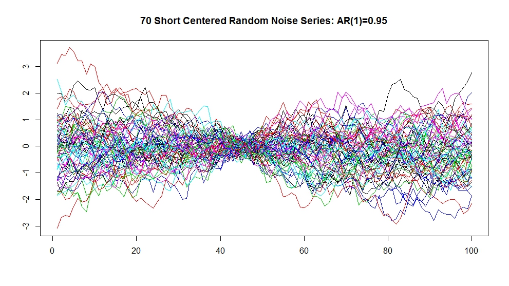 (http://www3.picturepush.com/photo/a/12651161/img/Anonymous/short-centered-random-noise-series-AR1-%3D-0.95.jpeg)
This graph
Looks like the sort of spread we would get by anomalizing individual realizations or temperature from a GCM. They would represent what happens to the spread in temperature anomalies when those anomalies are defined over a baseline.
But there is no “measurement error” in that problem because each realization of a GCM is a 100% correct rendition of itself. If run 1 of GISS EH has already been performed, there nothing random or stochastic associated with answering the question “What was the annual average temperature in 1980 for run 1 of GISS EH?” The temperature is what it is– you just compute it. Likewise, you can pull together many runs and get spreads on the anomalies.
But this has very little to do with the question in Marcott where one is trying to use proxies to measure the temperature of the earth. And so, presumably this figure is trying to tell us the range of possible temperatures for the earth based on the uncertainty due to both our ability to pull that temperature from a proxy and the fact that we selected a specific set of proxies.
If the figure immediately above is supposed to tell us the uncertainty in our knowledge of the earths temperature arising from the finite number of proxies there is no reason for the dimple.
Lucia:
–
Yes I have seen the short centered baseline “trick” that Gavin uses at RC with the model updates. As near as I can tell, there is no reason for short centering the model runs when comparing to observations. Model runs cohere misleadingly (dimple) in the short centered calibration range and increase the dispersion outside of the range.
–
Actually, when considering the “dimple” artifact, there isn’t much difference between the GCM model runs and the Marcott proxy measurement error because each is characterized by an independent random element which is an essential “dimple” recipe ingredient.
–
I am very interested in the nature of the “noise” or “measurment error” component of proxies used in climate reconstructions. To say in general that it tends to be autocorrelated would be an gross understatement. Back when the Gergis kerfuffle was going on I took a look at the screened proxies which Gergis used and resolved the simple equation of Proxy = signal + noise by subtracting the calibration signal (which was assumed to be without error) from each proxy presumably leaving the noise component. Rather than being 0 mean stationary random gussian noise as would have been assumed, these series were characterized by frequent mean shifts and were almost random walk like in character. Since they were screened against a calibration signal with a trend – surprise, surprise, the method pulled out the proxies containing biased noise with a slope in the same direction as the calibration signal. When one summed and averaged the selected proxy noise series, the composite noise was virtually a straight line trend! I was hoping to clean it up and perhaps post it up at Jeff’s blog but I just haven’t had the time. I have done one post at Jeff’s and I have to say that it’s one thing to play around with this stuff, but it is another to prepare a post. I admire and appreciate the work my favorite blog author’s put into their posts!
Not having fully digested Marcott’s work, I wouldn’t want to comment much on Marcott’s methods to produce that uncertainty graph other than to say that I agree with Steve M and others that it is obviously an artifact of short centering and is a misrepresentation of true uncertainty. After reading Roman’s post, I don’t hold much hope that even the dimple as an artifact is represented correctly in Marcott’s uncertainty graph.
LL (111923), I don’t agree. I think the issue is in making the transition from (biased) variance to measurement uncertainty.
I also think Lucia’s comments on how to do this are spot on.
Maybe I am misunderstanding you Carrick. When you state:
I read this to say that short centering where N=1 causes 0 variance in the case of sample variance but not measurement error.
But presumably the decomposed set of proxy measurement errors is independent, random, and stationary, no? If I define my white noise simulations as this set of random measurement error, and short center on an interval of N=1 I get the following. Where am I going wrong?
LL– It’s quarter to five. I’m outlined what figures to make to explain. I’ll post tomorrow. I’ll try to also explain the difference between the problem you and likely Nick are thinking you are looking at and how that differs from the uncertainty in determining the temperature from the proxies. Of course… I haven’t done the monte carlo yet. So maybe I’ll figure out I’m wrong. But I don’t think so.
Does anyone know what Nick is sayinhg here? Apart from an oddly desperate need to support a paper that has been thoroughly dismembered by everyone apart from Tamino who has invented a new way of interpreting the proxies in order to “support” (a new way of saying undermine) their conclusions.
Sorry I linked to the autocorrelated noise, rather than the white noise in the last post. This is the white noise N=1 short centering. It is harder to see but still unmistakeable.
re: lucia (Comment #111929)
Looking forward to it Lucia!
Neils, You are right about the comments at Real Climate. I was looking at a new thread which didn’t have any comments yet. They seem to be doing movie reviews regularly now.
Layman, It’s certainly possible to constrain a series of curves to individually pass through a single point, but that doesn’t tell you anything about the measurement uncertainty of the ensemble.
Let’s take an example where each curve has a known measurement error sigma, which is constant within each curve, and equal between proxies.
In this case, assuming uncorrelated errors between proxies, the measurement error is just sigma/sqrt(70), and unaffected by the centering technique.
The issue comes up with what happens when you try to use the variability between series to estimate the uncertainty. For this case, I suspect one can develop a quantitive formula for the unbiased uncertainty estimate of the anomalized temperature as a function of N, and from previous experience it will probably end up with a “zero” in the denominator associated with bias correction. However, it’s probably easier to just correctly model the temperature with a Monte Carlo to start with.
I don’t think Marcott did this part remotely correctly, though a fair amount of guesswork is needed due to the fact they haven’t provided code.
Let’s see what Lucia cooks up.
Layman Lurker, actually this case appears easier than I thought, and doesn’t involve any divide by zeros, unless you try estimating the uncertainty at a given time from the expectation value of the variance at that time. While this is unnecessary in this case, it does appear to be Nick is trying to do effectively by arguing that the measurement error is zero for N=1. Anyway, this should lead to a divergence at the intersection point when N=1, but it’s back-a**ed and unnecessary.
The measurement uncertainty for time “i” of the average of the proxies is,
$latex \sigma_i = \sqrt{\sum_{p = 1}^P (x_{ip} – \bar x_i)^2/P (P-1)}$.
where $latex x_{ip}$ is the value of proxy “p” at time “i” and $latex \bar x_i$ is the arithmetic mean over proxies at time “i”. This includes a correction for the error of the mean of $latex 1/\sqrt{P}$. (The uncertainty of individual measurements is a factor of $latex\sqrt{P}$ larger.)
Suppose we decide to anomalize this data, relative to some baseline range of $latex [i_1, i_2]$ and let $latex N = i_2 – i_1 + 1$. This involves subtracting a constant $latex x_a$ from each value.
I think Nick is using the definition:
$latex x_a = \sum_{i=i_1}^{i_2} \sum_{p=1}^P x_{ip}/(N \, P)$.
This has an uncertainty of
$latex \sigma_a = \sqrt{\sum_{i=i_1}^{i_2} \sigma_i^2}/N$,
by the quadrature rule, so the anomalized value at time “i” is
$latex \hat x_i = x_i – x_a$
and the associated uncertainty is
$latex \hat \sigma_i = \sqrt{\sigma_i^2 + \sigma_a^2}$.
Note in the case that Nick specified, where the measurement error is a constant $latex \epsilon$, then
$latex \sigma_i = \epsilon/\sqrt{P(P-1)}$,
$latex \sigma_a = \epsilon/\sqrt{N\,P \, (P-1)}$
and $latex \hat \sigma_i = \sqrt{1 + 1/N^2}/\sqrt{P(P-1)}$.
Caveat: Late at night, been dealing with signal-processing noobs all day, so if this is all hair-ball, the cat gakked it up.
Assuming I’ve done my cyphering correctly, the last equation should read:
$latex \hat \sigma_i = \epsilon \sqrt{1 + 1/N^2}/\sqrt{P(P-1)}$.
(I left out an $latex \epsilon$.)
Here’s another way of looking at the original problem. Why would just taking anomalies of a whole lot of proxies about an anomaly base cause a dimple™ CA in the CI?
Again, consider M (large) realizations of a “proxy” consisting of unit white noise only. CI’s would be &plusmin;1.
Now take anomalies over a base of N points (can be thought of as consecutive). Let S be expected sum of squares for that block. Then S=N*M
ANOVA – S is equal to the sum of
S0 = N * (sum of squares of each mean about 0)
S1 = the sum of M sums of squares about each respective mean.
Now for each mean in S0, the expected value is 0 and the variance 1/N. So expected value of S0 is N*(M/N) and so of S1 is M*N*(1-1/N)
When anomalies are taken, all the means are set to 0, so the sum of squares about 0 becomes just S1. And this must be the square of the average CI for the block. But it’s white noise – all points are equal, so to get the expected value divide by M*N, and take sqrt
CI=&plusmin;sqrt(1-1/N)
Elsewhere the same argument as before. You’re subtracting a mean which is an independent rv variance 1/N. So the variances add (independence), and the CI there is sqrt(1+1/N).
An interesting more advanced problem – if you look at the CA dimple, it’s pretty much quadratic. What happens to the above analysis with AR(1) noise? I think that would be pretty much quadratic. You could (after calculation) use this to estimate the effective lag.
Nick, serious question.
Are you actually arguing a position you believe yourself?
Please be truthful in your response.
Nick–
By using anomalies and a baseline, it is possible to create things that have a dimple. Those things don’t happen to be the uncertainty in the reconstructed temperature based on the proxies.
Carrick, IIUC your definition as per:
x_a = \sum_{i=i_1}^{i_2} \sum_{p=1}^P x_{ip}/(N \, P)
is wrong. Each proxy series does it’s own anomaly calculation subtracting it’s own baseline mean. Uncertainty is done at each time step.
–
Note, this is where my support with Nick ends on this. The dimple is an obvious artifact and should be interpreted accordingly.
Lucia,
Well, I’ll look forward to seeing that explained. Hopefully a toy reconstruction. Maybe Carrick could give one too.
I think the one I described above indeed is a recon, trivial of course. And it’s done exactly in the style of, say, Loehle and McCulloch. The CI’s are the pointwise sd’s (or 2*sd or whatever) of the anomalised proxies.
It’s midnight here, so I’ll be fading out soon. But yes, Carrick, I always say what I believe and believe what I say.
Just to back up LL on that, on line 93 of the Marcott SM:
4) The records were then converted into anomalies from the average temperature for 4500-5500 yrs BP in each record, which is the common period of overlap for all records.
That’s before any averaging is done. There are 73000 records each treated that way.
Nick–
I coding R right now. I want to show the uncertainties in the reconstruction and the ‘thing’ that contains a dimple.
Lucia,
If I could lodge a preemptive question:
“If the figure immediately above is supposed to tell us the uncertainty in our knowledge of the earths temperature arising from the finite number of proxies there is no reason for the dimple.”
Could you, in the post, be rather specific about what you mean by earth’s temperature and how it might be calculated? Most familiar measures, like GISS etc, are average anomalies (with a fixed base and, if you look into it, a dimple). And both GISS and NOAA have an explanation of why it has to be that way.
Nick–
I plan to be specific about the earth’s temperature and what it is. I will show graphs both raw temperatures and anomalies.
I would also say
“If the figure immediately above is supposed to tell us the uncertainty in our knowledge of the variations in earths temperature anomaly with time arising from the finite number of proxies there is no reason for the dimple.â€
I see the Marcott dimple as an artifact of using a “short centered” anomaly. I am not sure what this means to others commenting here or at CA other than something of which one should be aware i. e. it is an artifact.
Layman Lurker (Comment #111926)
“I am very interested in the nature of the “noise†or “measurment error†component of proxies used in climate reconstructions.”
I am always interested in seeing any analysis of proxies used in reconstructions since it is the proxies that are the basis of the reconstructions’ validity. If you do not start with proxies that are reasonably and faithfully responding to temperature the discussion of methods for manipulating the data becomes academic.
I have been looking at the Marcott proxies, as I described over at RomanM’s thread at CA, in attempts to determine whether the difference I see in proxy mean temperature changes over millennium time periods are statistically significant where the proxy are located in the same or close proximity. I have yet to finish my calculations, but the results will be very different using RomanM’s and Marcott’s calibration errors. I think my take away will be you cannot have your cake and eat it too, i.e. you either have very wide CIs on the reconstruction or face the fact that the proxy responses are statistically different.
Layman Lurker,
I’m pretty sure it reduces to the same calculation for the mean of proxies. Let $latex x_{ip}$ be the series in time “i” and proxy number “p” with a fixed uncorrelated Gaussian measurement uncertainty $latex \epsilon$.
The arithmetic mean of this series over proxy number is:
$latex \bar x_i = {1\over P} \sum_{p=1}^P x_{ip}$,
with associated measurement uncertainty given by the error of the mean,
$latex \sigma_{\bar x} = \epsilon/\sqrt{P}$.
Define
$latex \hat x_{ip} = x_{ip} – x_{ap}$
as the anomalized version of series, where
$latex x_{ap} = {1\over N} \sum_{i=i_1}^{i_2} x_{ip}$.
Then,
$latex \hat {\bar x_i} = {1\over P} \sum_p \hat x_{ip} = \bar x_{ip} – {1\over P}\sum_p x_{ap}$.
For brevity, I write this latter expression as $x_a$, where,
$latex x_a = {1\over P}\sum_p x_{ap} = {1\over N\,P} \sum_i \sum_p x_{ip}$.
Make sense?
Incidentally, given a uniform error $latex \epsilon$, the error analysis is straightforward from this point.
It’s really okay to agree with Nick here. 😉 I really am interested in the truth here, not engaging in blog wars.
You should use an error analysis of this sort to test and correct (really “calibrate”) methods that use analysis of variance to estimate uncertainty, since you “know” what it is supposed to be ab initio in this case. I can expand on this, but I think getting agreement that, given the assumptions I’ve made, I’ve arrived at the correct location would be useful first.
Nick thanks for the response.
I also detected a bit of cat gak in my previous analysis. If I get a chance, I’ll post a corrected version (or make fixing this as a homework problem, like one of my professors did when we noticed an error in his derivation 😛 ).
Whew… that took a while. Now I need to write it up. I want to exercise first though. So… tomorrow. But I now do have graphs of what the real errors are and so forth.
Carrick–
That sort of thing is borderline fair in grad school. It’s generally way out of line in undergrad. It’s also a horrible waste of time for the undergraduates since generally, they really do need to cover very specific stuff to do well in follow on courses. So if you let the syllabus slip.. gak!
Lucia:
I agree with this statement as long as we all keep straight it’s measurement uncertainty that doesn’t have a dimple and not the variance of the ensemble or series
The variance of the series should get smaller when you are in the baseline region, precisely as a consequence of the anomalization process. So dimple in variance, yes. Dimple in measurement uncertainty, no.
I added a brief comment here on this topic.
Briefly you’re by construction building in a correlation in the residuals, so you can’t simply use sum of squares of the residuals to estimate measurement uncertainty: The assumption of independence is now violated.
Agreed. To understand why and where a dimple appears you need to recognize the difference between the measurement uncertainty and the mere variance of a series that has been rebaselined. They aren’t the same thing.
does this mean, in layman speak….the errors should not reduce for any specified period unless there is a real reason why we know those measurements are more certain?
lucia (Comment #111958)
“Agreed. To understand why and where a dimple appears you need to recognize the difference between the measurement uncertainty and the mere variance of a series that has been rebaselined. They aren’t the same thing.”
I would hope that those who might appear to be disagreeing over this issue would agree with this statement – an artifact is an artifact and in this case of baselining.
Re: lucia (Apr 10 14:20),
Hooray! Exactamundo. I continue to believe we can all eventually come to agreement on this.
Perhaps these kinds of things need to be calculated in two columns. The data transformations in one, and the uncertainty calculations in the other, both in parallel…
“To understand why and where a dimple appears you need to recognize the difference between the measurement uncertainty and the mere variance of a series that has been rebaselined.”
Well, the “mere variance” was the basis of the CI’s in Marcott et al, and in Loehle and McCulloch, and in most others AFAIK. If you have a different measurement uncertainty, that implies you have some better way of measuring. I’m all ears.
Lucia: Would it be possible to set the dimple discussion as a separate post, perhaps starting with Carrick’s comment? The discussion is referenced at CA but is invisible to latecomers.
It is not a different measurement uncertainty. What you’ve done is define the uncertainty to be zero, which we know in advance is incorrect.
AFAIK the experts in each arena of proxy measurement provide their own estimates of measurement uncertainty, along with insight into other potential confounding factors (ie additional uncertainties). At the very least these tell us that uncertainty cannot be ignored nor arbitrarily set to zero. Hopefully we can agree on that! There should be nothing embarrassing about admitting what we do not know, or admitting that some uncertainties are potentially quite large.
I’m gonna sit back with the popcorn now and see what Lucia comes up with 🙂
bernie–
When I create a post discussing ‘the dimple’, I can move comments there.
Nick–
Once can compute the variance of all sorts of things. To be confidence interval, it has to be a variance of a specific thing.
Different measurement uncertainty? The thing called “measurement uncertainty” with the dimple is not the “measurement uncertainty” because it is a variance of the wrong thing. It has weird properties. This has very little to do with measuring.
I’ll be posting later. If it’s any consolation, if you make the dimple disappear, the computed confidence intervals are tighter (and have more desirable properties.)
Mr Pete: 6 Graphs. Some Latex. Can show why dimple goes away– and get uncertainty intervals that make sense and have decent properties.
http://www.skepticalscience.com/marcott-hockey-stick-real-skepticism.html
http://www.skepticalscience.com/marcott-hockey-stick-real-skepticism.html
Nick Stokes, “If you have a different measurement uncertainty, that implies you have some better way of measuring. I’m all ears.”
A better way of compiling the data really. Uncertainty should increase with time. Use the most current period as the baseline.
Brandon–
That is so weird. Instead of trying to tell us that Marcott is correct (or admitting that the criticism of the paper has been confirmed as largely correct), SkS is trying to explain “why skeptics should ‘like’ Marcott”.
They also kill a lot of strawmen. Among them, they imply that somehow criticizing Marcott is somehow actually advancing the argument climate sensitivity is high. Example “they’re also arguing that the climate is more sensitive than the IPCC believes.” Well…. sorry buddies. One can comment on the deficiencies in Marcott’s statistics without making any claims about the magnitude of climate sensitivity.
Brandon (#11970 & #111971) –
From the SkS article: “It’s understandable to look at ‘hockey stick’ graphs and be alarmed at the unnaturally fast rate of current global warming. But in reality, the more unnatural it is, the better. If wild temperature swings were the norm, it would mean the climate is very sensitive to changes in factors like the increased greenhouse effect, whereas the ‘hockey stick’ graphs suggest the Earth’s climate is normally quite stable…A ‘hockey stick’ shape means less past natural variability in the climate system, which suggests that climate is relatively stable.”
SkS is arguing that the hockey stick shape — in particular its smoothness except for the 20th century uptick artifact — is evidence that natural variability is low. Despite the fact that the reconstruction is guaranteed to be smooth by both the resolution of the proxies and the dating jitter.
In the words of Mr. Spock — may he live long and prosper — “Fascinating.”
dallas (Comment #111973)
“Use the most current period as the baseline.”
The problem is that a lot of proxies don’t have data in the period. I’ve put up a post here which tries to explain various things about anomalies – why use them, why you need a base where all proxies have data (or make elaborate correction), and it goes on to put theoretical CI’s on Layman Lurker’s AR(1) example.
Nick, anomalies with instrumental temperature and proxy temperature estimates are different critters. You can’t assume that proxies are unbiased, since they all are actually biased.
I am big into ocean reconstructions and noticed some irregularities with the physical ocean bottom depth of the core samples.
http://www.clim-past.net/9/859/2013/cp-9-859-2013.html
It turns out I wasn’t the first. So many of the ocean SST reconstructions are more likely ocean current reconstructions than true “temperature”. If you start with the most recent data and work back in time, you have a better change of building a better reconstruction and noting irregularities in the proxy data.
I have already done it, but you can try a present to 0 AD baseline, then use 2000 year baseline periods back to the beginning of the holocene. Does it make a difference?
I even picked a few of the proxies just for the Atlantic and Atlantic polar influences and used ~20ka as the start.
http://redneckphysics.blogspot.com/2013/04/playing-with-proxy-reconstructions.html
Imagine that, about 21000 years ago some of the proxies converge. Since I am not a statistical Guru, all I can say is that with an ~21,000 year precessional cycle, it would be reasonable to expect proxies of the past to contain some of that information if the choice of baseline is reasonable.
lucia, HaroldW, my favorite part was it saying Tamino is an example of real skepticism.
Brandon (#111978) –
I agree. It was amusing seeing them tell us what real skepticism looks like.
Well, I suppose it would be a real coup of framing if SkS & Tamino can define the “skeptical” view. We’d have to find a new moniker.
Nick–The difficulty is that in your analysis T is not “the error in the reconstruction”. So, the sd(T) is not the uncertainty in the reconstruction. The error in a reconstruction should be (Tearth-Treconstructions ).
This is true whether you use anomalies or not. To compute the spread in the error, you need to take a difference between what the thing you want to estimate and your estimate.
I had anticipated a slightly different issue, so I’m trying to see if this makes a difference to the argument. Maybe it will…. or not!
Ok… I need to tweak my examples to apply to what Nick actually did instead of what I thought he might be doing. Shouldn’t take too long. But it’s better to write the correct post. 🙂
(Sorry for promising to write and waiting. But until Nick wrote up I wasn’t precisely sure what he was doing. My example did capture an element of the problem. But it didn’t precisely engage what he is doing.)
Lucia, I have been attempting to make sense of the CIs calculated by way of Monte Carlo simulations in the Marcott paper and as critiqued by RomanM over at CA. I asked some questions over there of RomanM, but I think he has been off line for awhile now.
I think more important than the dimple, which is a rather simple thing to account for, is to understand on what the CIs in Marcott are actually based. It would appear to me that the CIs must be based on some 20 year average proxy temperature. Since the reconstruction has a 0 variance for periods of less than 300 years I am not sure what CIs based on 20 year periods means or how one would relate that to shorter or longer periods.
I have been attempting to determine whether the millennial average temperature differences from proxy to proxy are statistically significant. In the meantime I am attempting to do my own Monte Carlo simualtions in order to obtain Marcott reconstruction CIs. Mine are much different, but then I am not sure that I am comparing CIs over the same time period of averaged temperatures as Marcott did.
Interesting that without the smearing that Marcott does in his calculations a more or less random sampling using the Marcott sampling count would cover something less than 25% of the years of the reconstruction.
Ken:
The cause of the dimple, and why it is not measurement uncertainty ought to be rather simple. But as you can see, Nick seems to continue to believe it has something to do with measurement uncertainty. I’m focused on that now and I’m going to write a post up on that subject.
For the time being, I am not going to look into other issues.
Well, Lucia, here we go again giving Nick special attention. I hope he appreciates it. I don’t do emoticons.
Kenneth–
Believe it or not, this is giving Carrick special attention. I do do emticons, so :).
lucia (Comment #111987)
OK, Lucia, just so I know who the teacher’s pets are at the Blackboard.
” I do do emticons”
I do dimples 🙂
I’ve put up another post using AR(1) to get a dimply dimple.
Nick–
I read it. I decided to adapt my example to the what you really argue instead of what I thought you did. But I do have one specific question that isn’t very important but which makes a difference in terms of detail. I’m going to email you.
Kenneth Fritsch, I know, right? It’s not fair to the rest of us!
Oh… I read the previous one.
I think Kenneth likes it better when we restrict the conversation to exchange rates between quatloos and other faux currencies. 😀
Nick, I looked at your posts. I was going to comment on Nick’s thread, but it started looking like a manuscript on measurement theory, so I stopped….
I see three substantive problems here. The list is growing. >.< <– gratuitous emoticon
The first is not groking measurement error.
A second issue is not understanding that when you anomalize a series, you introduce a relationship between the residuals used to compute the variance that only vanishes when the error in measurement for the year in question becomes uncorrelated with the error from the baseline series.
However, the formal relationship between variance and measurement uncertainty Nick is trying to use to compute CIs is only correct when the residuals are completely uncorrelated.
Finally when one computes an anomalized series, it is understood that this equation holds for the expectation value of the quantities, rather than the measured quantities from a particular set of measurements.
To give a simple example, suppose we baseline the temperature with respect to 1960.
Then $latex \hat T (t) = T(t) – T(1960)$.
This statement is understood to hold for the expectation values of $latex T(t)$ and $latex T(1960)$, just as if you wrote F = m a.
(Newton’s second law is exact if the measured values of “m” and “a” are exact, and it makes no sense to define a different “F” that is “exact” for a measured set of “m” and “‘a”. The expression for anomalized temperature, for good reason, is not given a special pass here.)
Thus, when we construct $latex \hat T(t)$ from measurements, it is understood this is an approximation that is presumably converges to the “true value” as the number of measurements increases to infinity..
It easy enough to construct examples “where this matters”, for example, compare the expectation value of $latex (\hat T(t_2) – \hat T(t_1))^2 $ versus $latex (T(t_2) – T(t_1) )^2$. Assume an uncorrelated, uniform measurement error $latex \epsilon.$
Does anything special happen at $latex t_1= 1960$?
Unfortunately this is all I have time for.
Carrick,
“However, the formal relationship between variance and measurement uncertainty Nick is trying to use to compute CIs is only correct when the residuals are completely uncorrelated.”
I’m trying to show how dimples arise in the way Marcott et al, and many others, have calculated CI’s. I’m not propounding my theory on how recons should be done, or even how CIs should be calculated.
Still, there probably could be better ways; in fact I can think of things I’d try. But I’m looking forward to reading other people’s ideas.
In terms of uncorrelated – my analysis assumes them uncorrelated across proxies but correlated over time. Hence the time covariance matrix K, which has a big role in the AR(1) analysis.
Nick–
Dimples can arise in confidence intervals for something. But what is that something?
Better ways to calculate confidence intervals for what?
You seem to keep missing the fact that confidence intervals must be confidence intervals for a specific thing. So, you can’t just say “These are confidence intervals”. You need to say what they are confidence intervals for.
The AR(1) issue, the anomalie issue and all these other issues can’t resolve arguments about what those confidence intervals apply to.
Nick:
If I get a chance, I’ll write up some notes that may give some ideas.
I think I have a good idea how to approach this problem, but I’m looking forward to seeing what Lucia does with it.
Lucia,
“You seem to keep missing the fact that confidence intervals must be confidence intervals for a specific thing.”
OK I should try again.
I’ve postulated a stochastic definition of a proxy (unit white noise etc, but in general covariance K over time).
I have defined a process for turning that into an anomaly (Matrix D).
I have calculated and plotted the expected standard deviation (and 2*) for the result of operating on the proxy with D.
Mathematically, it’s the sqrt of the diagonal of the matrix DKD*
Call that y
In an actual recon with P such proxies (realizations), the CI would be y/sqrt(P). Same shape. In any case, the y axis is arbitrary, reflecting whatever noise level was assumed in the example proxy.
You can call it that and it only proves that you are mistaken. The reason why is that Treconstruction-Ttrue is a “realization of the errror”. And to get the measurement error, we want the CI on the realization of the error.
You do have confidence intervals for something. But those confidence intervals aren’t confidence intervals of error. So, they aren’t measurement uncertainty.
In most situations, the difference doesn’t arise, but it does here owing to “the anomaly method”. Ordinarily, the purpose of the anomaly method is to make the specific baseline unimportant because the only thing you care about in interpreting changes in temperature. But you are shoving in the fact the baseline is arbitrary making its moving around contribute to the confidence intervals for your measurement error. That’s silly.
And your uncertainty intervals end up not behaving like normal ones.
Nick Stokes, CI=y/SQRT(P)
Exactly. With enough proxies you can have unbelievable accuracy. Doesn’t matter if they are right side up or upside down, you will get the same vanishingly small CI. Now we can move onto other stuff since climate is insensitive to anything but the number of measurements.
Lucia,
“we want the CI on the realization of the error.”
Well, you may. I’m trying to calculate the uncertainty of what they actually do calculate, which is anomaly. That’s the “thing”.
You can’t be uncertain until you have numbers to be uncertain about. So I’m looking forward to seeing what numbers you have in mind.
Nick–
You error is before your step I!! Stop believing that explaining your matrix algebra is a magic incantation that will make things right.
What is the proxy supposed to be a measurement of? (Answer: Ttrue).
What is the error relative to what it is supposed to measure? errorproxy=(Tproxy– Ttrue)
After that, you can propose a stochastic realization of the errors in the measurement. Then proceed. Because the confidence intervals for measurement uncertainty are the confidence intervals for the errors in the measurement.
Even though you seem to be refusing to discuss what measurement error and measurement uncertainty are, that’s what this argument is about. So:
1) What do you think the proxy is supposed to be a measurement of?
2) What do you think the error in a single proxy measurement is?
3) What do you think the definition of “measurement uncertainty” is? If it’s not the confidence intervals of the errors in the measurement then why is your definition better?
Lucia,
“Even though you seem to be refusing to discuss what measurement error and measurement uncertainty are, that’s what this argument is about.”
Then I’m not a participant. I’ve explained what I’m doing.
But If I see some actual numbers that I could try to work out the uncertainty of, then I’ll happily look again.
Nick, you and Lucia are way over my pay grade here, but it seems to me that what you’re doing is analogous to calculating a CI when you should be calculating a prediction interval.
Tower of Babel
Nick — There are times when your remarks illuminate important points in the topic under discussion.
.
Still, I usually skip your comments, because I’ve been burned so many times. Life is too short to devote a lot of effort to decoding someone else’s silliness.
It would be helpful if you were better at holding yourself to a “clear meaning” standard. The other literate, numerate ‘regulars’ at The Blackboard do this quite well. Example: Lucia’s #112001, supra.
You are the outlier.
Perhaps you are aware of this point, and your style results from a puckish sense of humor, or an intention to derail certain conversations, or a desire to demonstrate loyalty to a popular if beleaguered cause. Or maybe your personality is such that communication on technical subjects constitutes a genuine mystery. You’ve never addressed this point in a satisfactory way, and you won’t in this thread, either.
.
Your graphical presentation of the Marcott’s proxies was first-rate, and very helpful for visualizing the data that went into his reconstruction.
Amac,
I don’t see how I could be clearer. People compute anomaly means, and I’m calculating the CIs for that. I think that’s useful.
People don’t calculate temperature means, so i don’t know how to calculate CI’s for numbers I can’t see.
As you say, I’m the outlier. I’ve produced actual numbers and actual CI’s for them. No-one else has.
Nick
You mean you’ve explained the matrix algebra you pushed numbers through. That’s a rather limited sense of the term ‘explanation’. Because you are leaving out what the resulting product describes.
Yes. You seem to be focused on replicating a feature of their graph using a toy example. You seem to avoid discussing what the graph represents either in your toy or in their paper. But no one should care about the graph or the details of how it is created if you don’t know what it represents. (Or if the answer is: My replication represents the graph they would have made.)
But in your post at CA, you linked a whole bunch of people in your post and are involved in an argument about what those computed uncertainties represent.
For example: at climate audit, you responded to Terry
with
So why don’t you tells us your answer to “of what”?
Because whether you wish to believe it or not, you are partaking in a discussion where lots of people are arguing about the “of what”. And I’m telling you they are not uncertainties in the measurement of the earth temperature. They are also not uncertainties in the measurement of the earth temperature anomaly.
What do you think the “of what” is for the Marcott temperature anomalies? Or if you wont’ answer that, do you think knowing “of what” is unimportant? Or irrelevant to understanding or interpreting Marcott’s figures? Because you sure seem to be refusing to answer the question “of what”.
It’s all well and good to keep trying to dodge the question about the “of what” by showing matrix algebra to show they are confidence intervals of something. But you know… the “of what” actually matters if you are going to figure out how they should be used or interpreted. If you don’t know or refuse to answer the “of what”, you are presenting confidence intervals that are not worth looking at because you don’t know what they are telling you about anything.
Ok.. back to growling at latex…
Lucia,
It’s late here, but I’ll just offer one more thing. I don’t think CI’s belong to things. They belong to calculation processes. You start with data with uncertainty that usually have to be considered given. You process the data and generate numbers. The calculation process, and the data, create the CI’s for those numbers.
I’m describing the CI’s associated with the anomaly calculation process. If there’s a satisfactory temperature calculating process, fine, I’ll switch to that. As I said, I’m all ears.
Nick
If you don’t think they belong to things that’s explains a lot. It means you don’t understand what they are. If they don’t belong to things they are useless.
There isn’t any calculation process that resolves this problem. You need to go back to square 1 and learn the purpose of CI’s. When you understand that, you will see that how a CI should be computed depends on what it is supposed to “belong too”.
Nick —
> As you say, I’m the outlier. I’ve produced actual numbers and actual CI’s for them. No-one else has.
While you have produced numbers, that doesn’t make you an outlier. Read this blog for a while, and you’ll realize that you’re in good company there 😉
Anecdote time. When I was active in refereeing submissions for peer-reviewed journals in my field (biology), some of the first things I would check would be the error bars in figures. I was looking for answers to simple questions.
* Are the authors presenting standard deviations or standard errors?
* Can readers tell whether an error bar represents SD or SE?
* Which is appropriate? If there’s a non-obviously-correct choice, did the authors justify it?
Perhaps half of the manuscripts had problems. The most common issues were:
* Authors weren’t clear on the distinction between SD and SE.
* Authors preferred showing SE, because the error bars are smaller, making their graphs look more impressive.
You understand these simple issues. Yet you insist on idiosyncratic, non-intuitive meanings for commonly-used terms like “confidence interval.”
If everybody did this, the result would be another Tower of Babel.
I don’t think you would like me as a reviewer 🙁
I don’t think CI’s belong to things. They belong to calculation processes. You start with data with uncertainty that usually have to be considered given. You process the data and generate numbers. The calculation process, and the data, create the CI’s for those numbers.
Nick, I think you’re leaving out some things here. In particular, what do you mean by “things” in “CI’s belong to things”, and what do you mean by “numbers” in “generate numbers”?
If by “numbers” you mean parameters, then what you’re talking about are the SE’s of the parameters, which do (mostly?) reflect the process used to calculate those parameters. If this is what you mean, then the SE’s can be said to “belong to” the parameters. They arise because of how you calculate the parameters, true, but they describe your uncertainty — given your process — of the parameter values.
Lucia, Nick’s reasoning has brought to mind an analogy that I can’t shake. Say you’re in the field measuring the weights of coconuts. You then want to calculate the average weight of those coconuts — not yet trying to generalize beyond your sample. If you want to allocate the uncertainty of your average, I could think that it’s associated with your process (the scale and your attentiveness) rather than with the coconuts themselves. If by “things” Nick means coconuts and by “things” you mean the scale, which Nick would call the “process” rather than a “thing”, could that be the root of the misunderstanding?
As the novice that I am, it feels like Nick’s view — as I understand it — is reasonable: that uncertainties are associated with processes not objects. Though I think he’s isolating one part of a longer process and calling it The Process and thus ignoring important sources of uncertainty on the way from data to conclusion.
Nick says, “I don’t think CI’s belong to things. They belong to calculation processes. You start with data with uncertainty that usually have to be considered given. You process the data and generate numbers. The calculation process, and the data, create the CI’s for those numbers.”
Nick, I think you’re leaving out some things here. In particular, what do you mean by “things” in “CI’s belong to things”, and what do you mean by “numbers” in “generate numbers”?
If by “numbers” you mean parameters, then what you’re talking about are the SE’s of the parameters, which do (mostly?) reflect the process used to calculate those parameters. If this is what you mean, then the SE’s can be said to “belong to” the parameters. They arise because of how you calculate the parameters, true, but they describe your uncertainty — given your process — of the parameter values.
I also suspect that by “things” you mean data, while Lucia might mean something different.
Lucia, Nick’s reasoning has brought to mind an analogy that I can’t shake. Say you’re in the field measuring the weights of coconuts. You then want to calculate the average weight of those coconuts — not yet trying to generalize beyond your sample. If you want to allocate the uncertainty of your average, I could think that it’s associated with your process (the scale and your attentiveness) rather than with the coconuts themselves.
I think that Nick is accounting only for the middle part of a process and not the entire process from start to conclusion. In that sense, the “thing” at the end of the process is a statement about tempe
Lucia, sorry I tried to edit something and now it appears there are two copies and the “wrong” one won’t delete and I can no longer edit the “right” one, which lost some stuff at the end.
Wayne2
Your missing something: A calculation process has to operate on numbers generated by something. What “thing” the CI belongs to depends on the “thing” your sample data represents before you throw it into the calculation process.
If you stuff in weights of coconuts into your averaging operator, the average will be the average for coconuts not for apples or pears. So, the average you compute must apply to this “thing”:
If you find yourself unwilling to admit that the average applies to coconuts and start claiming it’s ‘just an average’ or that “averaging is just a process’, then you are forgetting about an important characteristic of your average: It applies to coconuts.
By the “thing” I mean: I want to know “data describing what thing“. When when someone hands me an “average” that is spit out by the “averaging process”, I want to know wither the input data was weight of coconuts, weight of grapes, weight of American men or what. So it seems to me the conversation with Nick goes like this:
Lucia: “What thing do these confidence intervals apply to?”
Nick: “They are just confidence intervals”.
Lucia: “Confidence intervals for what“?
Nick: “Confidence intervals are just the output of a process. They’re just confidence intervals. I’m just showing how Marcott would get them. My matrix algebera is okey-dokey. I used AR(1) noise. Look I made a dimple! Kewl!”
Well: My claim is that Nick’s confidence intervals are not the measurement uncertainty for the earth’s temperature (anomaly or otherwise.) If nick wants to just keep saying confidence intervals are just confidence intervals shat out of some mathematical process fed with “data”, that’s all well and good. But if so, why don’t we just create a time series out of the weight of coconuts plucked from in Hawaii, run that through a processing box, collect the stream of ordure that comes out and call those “the confidence intervals (for some unstated thing which– evidently doesn’t matter because confidence intervals don’t apply to ‘a thing’)”
If you mean that the true uncertainty in the mean weight of coconuts is not a property of the specific coconuts you use to estimate the uncertainty, I agree with you. That’s not what this argument is about.
If you mean that the uncertainty in the mean weight of coconuts doesn’t depends on the property of coconuts themselves but could just as easily be determined by using data from apples, I disagree with you. In both cases, even though averaging is just “a mathematical process” the computed average applies to a thing. If the data were collected from a sample of coconuts that thing is coconuts. If the data were collected from a sample of apples that thing is apples.
My impression after a few years of looking in from the outside is that, as an institution, Climatology sees itself as being in a Special Snowflake situation when it comes to analysis of data. In particular, learning from the sophisticated work that’s already been done in other fields is optional rather than required.
I suspect that top-notch biostatisticians who design complex, expensive clinical trials would have a great deal of useful advice on how to approach the large amounts of time-series data that go into Marcott-style paleoreconstructions. But it seems as though they are never asked.
“There are different ways to think about variability and error, and multiple approaches, each suited to answering particular questions” is one of the underpinnings of diagnostic test design, evaluation, and interpretation. But each scientist who works on such a problem doesn’t publish based on his or her own quirky, idiosyncratic approach. That wouldn’t be sensible.
AMac–
Why you would expect biostatisticians to have expertise in time series data?
It’s certainly true that people in medicine are often going to be required to use pre-existing established methods to get approval for an experiment and to publish material that is going to be submitted to the FDA for a clinical trial of a new pharmaceutical or a new medical practice. But I don’t immediately see why this should generally involve time series nor any technique that would be important when creating a proxy reconstruction. This may be because I don’t know what bio-statisticians do– but what problems do you think the do that specifically involve time series and/or creating a proxy reconstruction?
> Why you would expect biostatisticians to have expertise in time series data?
Longitudinal studies involve following subjects over time, and collecting information at intervals — that’s what I had in mind.
I’m no biostatistician, but I’ve overall been impressed in my dealings with them. My suspicion is that climate studies could be improved by more rigorous application of principals that are widely used in other disciplines. It seems likely that there are numerous areas where time series are routinely analyzed, e.g. aviation, engineering, chemistry, and astronomy. I have little-to-no professional contact with people in those specialties.
Perhaps, as a rule, folks who competently apply statistics in those areas look over to climate science and say, “they do as good a job as we do.” That’s not my impression, but it could be so. In which case, I’m wrong.
I just saw a link in a “tweet” from John Cook I had to share. Two “tweets” before, John Cook gave a link to a Skeptical Science article about Marcott et al which said:
Shortly after saying a “result is probably not ‘robust,'” John Cook praised an article which depended, to some extent, on that result. The only reason the “projected temperatures” fit the end of the “reconstructed temperatures” well is because of the result John Cook’s site says is “probably not ‘robust.'”
What a crazy world we live in.
Speaking of which, what is up with the graphs in that piece? Am I missing something, or is the idea we’ll reach 900 ppm of CO2 by 2100 crazy? And why does it say:
Then show a graph which shows effective CO2 levels are just under 400 ppm yet jump up faster than CO2 alone can explain? CO2 levels are just under 400 ppm. If we take the effective levels of “the other important warming agents,” we should be well above 400 ppm.
It seems the graphs are actual CO2 levels combined with projected “effective CO2 levels.” Is that right? If so, how could John Cook be so blind as to praise the piece for its “powerful graphs”? Is he saying misleading graphs are good because they’re “powerful”?
Brandon (#112052)–
The Sokolov et al. paper on which the blog post is based, arrives at a mean estimate of 900 ppm CO2 by 2100. As far as I can tell, the primary reason is the claim that natural CO2 sinks will become less effective over time, due to the hypothesis that plants will become nitrogen-limited. See their figure 12 especially.
Since I’ve posted a few comments on SKS this last week, I got to see news everyone here should be interested in. UAH TTL may barely have budged up a smidge, but global warming is accelerating!