NOAA/NCDC published their April 2011 Temperature Anomaly rose to 0.5852 C relative to March’s 0.5103. I plotted temperature since Jan 2001 along with trends and IPCC projections for surface temperatures forced using the A1B scenario below:

Andrew Montford emailed enquiring for more detail on the information in recent graphs, all of which use the same convention. It’s easiest to explain using a shorter time period graphs which is one of the reasons I’m showing the shorter time period graph here. (The other reason is that I think projections should be tested against data that was observed after the modeling choices affecting the projections were already made, so prefer to not test projections against data that predate selection of the A1B SRES.)
The items in the graph are described below:
- Light gray erratic line: Monthly anomaly data from NCDC.
- Thick black trace: A smoothed multi-model mean of 22 models used by the IPCC to make projections. This trace represents results using A1B forcing. This is similar to the multi-model mean shown in the AR4 figure 10.4 in the WG1 Report. They smoothed their multi-model mean using some method; I applied 25 month smoothing to mimic that. Note that this sample mean is an estimate of force response averaged over the 22 models. (For discussion of the term “forced response” see Issac Held’s blog. )
- Light grey dashed line: The 1 σ range of temperatures from 25-month smooth model means from the 22 models used to create the multi-model mean. Figure 10.4 in WG1 of the AR4 also showed a 1σ range for the multi-model mean temperatures which they also smoothed. (Note: the order of operations can affect the spread of these uncertainty intervals. I applied temporal smoothing and computed the sd on the smoothed temperatures.)
In principle, this is an attempt to represent the spread of the forced responses from each of the 22 models which communicates something about the range of uncertainty arising from modeling choices (e.g. parameterizations, forcing history, resolution etc.). In practice, it’s something a bit odd because some models only have 1 run and so internal variability of “model weather” also contributes to this spread.)
- Black dashed trace: The ordinary least squares trend line fit to the monthly values of the multi-model mean from Jan 2001 through April 2011. This happens to have a trend of 0.21C/dec, which is a bit higher than “0.2” contained in the phrase “about 0.2C/decade”.
- Red solid line: the best fit trend using ordinary least squares. Sharp eyed fans of negative trends will notice this is currently -0.003C/decade, i.e. less than zero. Don’t expect this exciting event to last past June. (Notice that the April anomaly lies above the trend line; if the May value equals or exceeds the April value, the computed trend will increase.)
- Red dashed line: The ±2σ uncertainty intervals for the trend computed by apply a red-correction to those estimated by ordinary least squares. When doing this I also made a slight upward correction for the estimate of the lag-1 auto correlation. The red-correction was used by authors of the AR4 to explain that warming in the thermometer record is statistically significant. It is also the noise model used by Santer when discussing tropospheric temperature trends. It’s a very popular noise model in climate science.
- Green solid line: the best fit trend using ARIMA(4,0,0). Some will wonder, “Why ARIMA(4,0,0)?” The reason is that owing to frequent complaints that it is difficult to identify the correct model type with short time series (which is true), I organized the script to hunt for the ARIMA(p≤4,0,q≤4) fit that gave the largest uncertainty in the trend of all possible fits of that form.
Fans of negative trends should note: This best fit trend is positive. 🙂
- Green dashed lines: The uncertainty in the trend estimated using ARIMA(4,0,0) to which I added the uncertainty based on the full range of trends from all ARIMA(p≤4,0,q≤4) models that R would produce trend.
Eagle eyed observes will notice the slope of the black dashed line corresponding to the best fit trend to the multi-model mean lies outside the range for the trends based on ARIMA(4,0,0). That is: 0.21 C/decade is greater than 0.118C/decade the largest consistent with this bit of data based on the assumption the residuals can be described using ARIMA(4,0,0).
- Green dashed curves: The uncertainty in the trend including both the uncertainty in the trend and the uncertainty in the intercept for the linear model through the data. The uncertainty arising from the intercept includes both the uncertainty based on the ARIMA(4,0,0) model but also the uncertainty in intercept from the baseline period.
Eagle eyed observes who understand how to interpret these graphs will notice the point in time where the red (or green) uncertainty intervals intersect with each other. The will notice that at that location in time, the black dashed line is outside the green dashed uncertainty intervals. This means the constant associated with the linear trends through the multi-model mean is also outside the range consistent with data. That is to say: The time average of the multi-model mean is higher than the observations and this difference is statistically significant.
- Purple curve: This is the 13 month centered average of the monthly observations. We’ve been noticing that since 2001, the peaks of the 13 month averages have approached and sometimes slightly exceeded the multi-model mean, but overall, the 13 month average remains below the multi-model mean. Currently, the 13 month observation mean lies outside the 1σ range for model-mean temperature; (i.e. the tip of the purple trace is outside the dashed grey line). What this means is subject to some interpretation because the earth temperature contains the stochastic variability associated with 1 realization while a portion of that has been averaged out of the spread of the model mean temperatures. (Also, one is a 25 month smooth and the other a 13 month smooth.)
- The graph includes a number of notes. I nearly always rebaseline data to ensure all comparisons are made on consistent baselines; the baseline I used is provided in the upper left hand corner. Because the baseline of 1980-1999 differs from the one used by NOAA, the anomalies in the graph are shifted relative to NOAA/NCDC reported values. Author and datasource notes are in the bottom left. The time stamp is placed in the lower right hand corner.
For those wanting a quick summary: If one accepts 2001 as a reasonable start year for analysis, and one is only considering NOAA/NCDC data, based on information in this graph only we would conclude that:
- The forced trend for the current period falls in the range of about -0.11 C/dec to 0.12 C/dec. (Knowing longer term trends are positive, I would bet on the upper range.)
- During the periods of projections, the multi-model mean of projections exceeds the observed temperatures reported by NOAA/NCDC and by an amount that is not consistent with observation based estimates of the stochastic variability of earth global mean surface temperature. ( Note: This finding pretty robust to start year. Using the ARIMA(4,0,0) fit and beginning analysis in 2000, the multi-model mean also falls outside the range consistent with the data.)
Since Jan 2000 Since Jan 2002 


Now: I’ll close with a bleg. All these figures are blurry. Does anyone have tips on the best method to generate R graphics that look clear after uploading to my blog? (The blog software shrinks the size. I guess I can pick larger fonts etc. But if people have examples that might help me find the most efficient method.)
Lucia, have you tabulated comparisons of trends using your recent calculations for different data sets; such as for NCDC, GISS, UAH, HadCru?
In some comments in blogland, it is averred that GISS is the outlier, on the warm side. Is that true? I seem to recall that you have made some comparisons in the past.
Humm…
Yet another indication that the models (circa 2001) are not a good representation of measured reality. I guess we have to wait for AR5, where I expect the 95% confidence limits on model projections will be expanded to include… well, to include most any plausible measured temperature data. It is so cool to be able to ex-post-facto show yourself correct, in spite of the data!
.
But a serious suggestion to Gavin and company: expand the uncertainty limits in AR5 to include measured reality…. then scale down your claims of catastrophe a lot, lest the next Congress choose to not fund your work.
Don B —
I believe you are looking for this post:
http://rankexploits.com/musings/2011/which-observation-is-the-outlier/
Although it does not include the satellite temps, since technically they are not measuring the same thing.
SteveF–
One thing to consider: The model mean does not include anything about the solar cycle. Those that did include the solar may have left their sun frozen on the relative high value at the end of 2000 when most groups end their 20th century runs. (Some end in dec 1999 at least one start later– like 2004 or so!)
I don’t know why the modeler’s didn’t agree to include some “average” solar cycle which might have resulted in a force trend with the average solar cycle showing. But they didn’t include any. So this may be part of the reason for the deviation. But given the tendency of many to insist that there simply is none, I like to keep the question of “is/isnot” we separate from “attribution”.
DonB–
My impression is a lot of people rooting for “no warming” want to just call whatever looks highest an “outlier” and those rooting for “lots of warming” want to call whatever looks coldest an “outlier”. But I don’t think we have enough data sets to decree any one of the surface metrics an “outlier” relative to the the other ones. In any analysis, one method gives the most warming; another gives the least, and one is in the middle.
Lucia —
My impression for the GISS model was that they used the 11 year solar cycle in their “Various Future Scenarios to 2100” based on the figures:
http://data.giss.nasa.gov/modelforce/solar.irradiance/
However, the forcing data itself only goes up to 2000, so perhaps not.
Lucia
Would you mind helping a dummy out? Your “Light gray erratic line: Monthly anomaly data from NCDC” has a final data point with abscissa (as close as I can make out) Month 4, 2011 (April 2011). So far, so good. The ordinate, however, of this point is about 0.28 (again, Mark I eyeball).
Yet you say “April 2011 Temperature Anomaly rose to 0.5852 C”
What gives? 0.28 plays 0.5852? What is this dummy missing?
Funny, but I (think I) understand the rest! 😉
Heretic– I’ve rebaselined. The baseline is provided in the upper left hand corner. I’ve been asked this before so I’ll add that!
Aha! Thanks for taking the trouble.
lucia (Comment #76050),
Fair enough, the solar cycle that peaked in ~2005 may be altering the surface temperature record significantly. But, the devil in me asks, what will happen as the current solar cycle ramps up? Are we going to see a renewed warming trend? My guess is, no, not very much; the 60-70 year 0.2 C AMO-like cycle suggests that the next 20 years will warm at only ~0.085C – 0.09C per decade, modulated by ENSO of course.
.
10 more years will resolve the question.
SteveF–
I’m not saying I think the lag is necessarily the failure to include the solar cycle. But at least hypothetically, this could be a reason. I know some papers suggest the solar cycle is detectable over noise. They strike me as doing a lot of ad hoc filtering/ picking etc. Mind you, they may be right– or not.
I haven’t seen much to convince me the solar cycle is really detectable over noise.
Admittedly, there must be some effect, so maybe it has been 0.1C peak to trough. Or not. We’ll see.
A very tentative suggestion:
Push 11. to 1.
png will look better for this sort of plot-like graphic; jpg is better for photo-like stuff
Lucia,
The PNG is the patent-free successor to the GIF format. PNG has lossless compression whereas JPG has lossy compression. For photos or photo-like images the lossy compression is a feature, as it allows for significant reduction in file size with imperceptible reductions to the image quality (as discerned by the human eye). That same compression applied to vector graphics results in smearing of colors at sharp edges, resulting in the bug-not-feature blurry images.
lucia (Comment #76050),
I know you don’t necessarily think that.
If the solar cycle is influencing current temperatures via a direct (as opposed to cosmic ray/cloud) effect, then we can make a reasonable estimate of what to expect. 1.2 watts/M^2, peak to trough in a solar cycle (in space) means ~0.7*0.25*1.25 = 0.22 watt/M^2 average surface intensity variation over a solar cycle. If equilibrium sensitivity is ~0.82 C/watt/M^2 (assuming the middle of the IPCC sensitivity range), and assuming the more-or-less immediate response is ~40% of that, we ought to see ~0.4* 0.82 *0.22 = 0.072 C variation over the solar cycle. If the sensitivity is on the low end of the IPCC range (~0.55 C/watt/M^2), then the immediate response must rise a little, and the solar cycle influence should be near ~0.06C. At the upper end of the IPCC range (1.23 C/watt/M^2), the solar cycle influence ought to reach ~0.1C, or a little less, depending on how much immediate response we believe would be present at such a high sensitivity. Below the IPCC range (like my personal estimate of ~0.45C/watt/M^2), the immediate response has to rise a bit, so the solar signal should be near 0.05C. So over a plausible range sensitivities, the solar cycle effect is ~0.05C to ~0.1C.
.
Seeing that smallish effect when there is 0.25C (+/- 2-sigma) variation around the secular trend (ignoring all longer term variation) would appear a challenge, but maybe with enough cycles it would be visible.
.
If someone claims a response of >0.1C, then either a) there must be an indirect (cosmic rays/clouds) solar effect or b) the real climate sensitivity has to be substantially higher than the top end of the IPCC range.
Starting in about 2000, GHG forcing drives the ensemble mean temperature forecast. I don’t see any variation from the other forcings showing up at all.
Starting in about 2000, the forecast going out to 2100 follows 3.89 ln(CO2-a1b) – 22.60C to the T. If you use a 24 month moving average of the forecast, it does not vary by more than 0.03C from this formula (I’m using the 1951-1980 base period so the intercept of -22.6 might change based on the base period used).
This also translates into a lag of just 5 or 6 years (from the instantaneous 3.0C per doubling value) out to about 2030, after which it starts increasing until it reaches a 13 year lag by 2100.
So much for all the magic “various forcings” and “long ocean lag” explanations.
It is CO2 all the way (other than the ensemble mean also predicts a large increase in the seasonal annual cycle – this does not show up in a 24 month moving average but does in just the monthly values).
http://imageshack.us/m/851/7545/ipcclagsurprise.png
Lucia,
FWIW, the correlation of sunspot number (1-year lagged) against Hadley temperature, Nino 3.4 and GHG forcing, also lagged, suggests a solar cycle effect (for a cycle of 150 sunspots) of about 0.055C +/- 0.042C (95% range)… consistent with almost any sensitivity one wants to claim.
Lucia, use png.
If you need sample code just ask
png(filename, ….)
plot(filename…)
dev.off()
Thanks for doing this Lucia. Hugely appreciated!
Never use jpg for any image with lines or text, because jpg smooths.
Sorry, I see I’m the nth person to say that!
Bishop – are you sending this to Hengist McStone?
Lucia, regarding your “bleg”
The thumbnails of the graphs are clear enough. As long as you have them hyperlinked to the full size graph, it works out just fine for me. You may want to test whether the blog software treats png’s differently, but I suspect you’ll see the same result.
A one of the 10% or so who are colour-blind, could I beg you not to use red and green (or blue and purple) lines in the same plot? It makes it nigh on impossible for me to determine what’s what!
mct–
Sorry. I’ve been trying to think of what color to choose. I have trouble seeing yellow. I’m not sure what that leaves. Can you suggest which colors are good? (Does it help if if it’s darkened? Like maroon? Etc.)
Lucia, can you try changing the dot-dash pattern as well as the color? I’ve found that helps a lot. (- – – – .—.— …. – — – — etc )
(This harkens back to the days when people only had black-and-white copiers and you had to make your graphs “black-and-white” proof.)
Also I’ve found this yellowish-gold color a good one for plotting lines, if you want something in the yellow family:
col=”#ffe737″
There’s a good calculator here too.
Carrick–
I’ll look up the line types in R. (I happen to think people should use color and line types– but I hadn’t looked up all the line types yet.)
The yellow gold looks good. What I noticed with pallette() in R is the first set of colors are all bad for the color blind!
Lucia,
Another option is line weighting. Thicker/thinner lines combined with different brightnesses (gray-scale weighting) and different dot-dash patterns should allow you to make graphs that even the unfortunates with some color vision deficiencies can figure out.
Just seein’ if my 3000 minutes are up yet. 😉
Happy Friday is this is allowed.
Andrew
Andrew_KY– I think it’s 150 minutes. But if there is a bug…well… there is a bug.
RE: SteveF (Comment #76066)
Steve I appreciate your careful analysis of solar TSI changes and resulting changes in W/M^2. Clearly these small changes do not account for the majority of warming during the CWP (current warm period).
My question? What are we missing? Not rhetorical. These small changes in TSI clearly do not account for the climate change over the last 2000 years that were strongly correlated with long term changes in solar activity. Evidence from NA and European glacier records suggest climate swings of +/- 2C. This is consistent with GISP2 ice core records as well. Measured changes in TSI simply do not account for these temperture swings and yet… they did happen.Is there some sort of compounding effect that results during periods of longer term (50-100 years) high or low solar activity?
HadCrut is out for April: 2011/04 0.405
….unfortunately they’re missing all of Canada in their analysis(http://www.metoffice.gov.uk/hadobs/hadcrut3/) which was below normal (see here: http://www4.agr.gc.ca/resources/prod/doc/pfra/maps/nrt/nl_mdnt_tmp_s_e.pdf)
FredN–
I know. NOAA, Hadley and GISS are all out.
I’ve been looking at a new test based on both the difference in the trend to a fit to the data and the intercept but I want to know the properties before writing up a blog post.
Also– I wonder why Canada’s data didn’t make it in. My impression is that’s unusual. OTOH, I haven’t kept track of which agencies report promptly and which don’t.
April is warmer than March? Who knew?
Other than being examples of high grade math and statistics [“negative trends” of -0.003C and temperature increases/decreases between -0.11 and +0.12/ decade] is any of this in any way shape or form conclusive evidence for the “A” in AGW/ACC?
Just asking, because isn’t that what the bottom line is all about? Not the ups and owns of whatever magnitude these may be, but their root cause?
tetris (Comment #76098) May 20th, 2011 at 10:56 pm
Well done tetris! At least someone (else) is looking at the wood in spite of the trees…
tetris–
There is nothing in a series of temperature data since Jan 2001 that could, by itself, conclusively prove the “A” in AGW. One would have to look at more data and other data. (Longer data series etc. Levels of CO2 etc.)
Anthony (Comment #76097) May 20th, 2011 at 9:42 pm
April is warmer than March? Who knew?
= = = = = = = = = = = =
The anomaly is greater. Do you not understand what this means?
dorlomin– I think it was meant as a light hearted joke.
Lucia, (Comment #76104)
.
You are correct with your first part. The trouble with the second part is that none of the ‘long term’ datasets are able to conclusively prove the ‘A’ either.
.
The longest running temperature dataset is the Central England Temperature data. The mean temperature for year 1659 is 8.83 deg C. The mean temperature for 2010 is also 8.83 deg C. No proof there (and I know England is not the globe, but if anyone can find a longer dataset from anywhere, please use it).
.
The 160 year-old HadCRUt dataset shows a 0.9 deg C (three year running mean) rise. At the same time, but not necessarily caused by, there has been a 40% increase in CO2 levels for what amounts to a 3% increase in global temperature. The trouble with that is no-one can say for sure that all the 0.9 deg C rise is due to CO2, or anthropogenic factors of any sort.
.
tetris’ comment is valid. The root cause is the bottom line, and needs to be proven.
Arfur–
Whether valid or not, I don’t know why tetris is asking the question. This post makes no claim about proving or disproving AGW. He can’t possibly learn anything about the plausibility of the AGW claim from this post. So asking whether it shows it or not? Why? Seems like some sort of non-sequitor type question.
tetris,
One way to look at it is as follows.
After a volcano we see a drop in temperature. Not big drops, in the vast
history of climate they are rather unremarkable. Still, we think
we have a physical mechanism which explains the drop. The emmissions
from a volcano change the radiative properties of the atmosphere. We can
build equations based on physical laws (theory) which describe how the temperature will change. These equations do a good, but not perfect job
of explaining the dip. Now, could the dip be cause by something else?
Sure. Logically speaking, it could be gremlins. But we have a phenomena
and we have an explanation, laid out in equations that use the physical
laws that we believe to be true. Physical laws that we use in everyday engineering.
The same goes for the temperature increase since 1850. We see a rise.
We see multiple lines of evidence for that rise: thermometers, ice retreat,
sea level rise. What is the cause of this. Now, here too we might note that the rise looks rather unremarkable. Much like the dip after a volcano looks unremarkable. Still, we can offer an explanation for this rise. The explanation
consists of equations. Those equations rely on physical laws. laws we use in
everyday engineering. What those equations explain is that a portion of that
rise can be attributed to increases ( and decrease) in certain forcing agents,
C02, methane, black carbon, aerosols and internal variability. Could be be something else? Sure, logically speaking it could be gremlins. If we want to
REPLACE the current explanation ( its GHGs) then we need a better explanation. we need a better set of equations that also use known physical
laws. Absent that better explanation, we are left with the explantion we have.
And note “natural variation” is not an explanation. It is the absence of an explanation. it is the absence of equations that rely on physical laws.
“And note “natural variation†is not an explanation. It is the absence of an explanation. it is the absence of equations that rely on physical laws.”
Amen.
And let’s say we have a set of equations partly based on physical laws that are trying to explain some aspect of physical reality.
Physical reality however does not match up with the equations.
Therefore, we ignore physical reality and continue to rely on our set of equations that are only partly based on physical laws.
For example, how many Watts/m2 does it take to increase Earth’s temperature to 291K from 288K.
There is a well-known equation which is very successful in explaining radiation and temperature across the universe for everything that we look at. Yet it is not used in climate science in determining how many Watts/m2 it takes to raise Earth’s temperature to 291K. A made-up guess is used instead and the climate models are programmed with that guess.
And, “natural variation” – Do you deny that the unforced natural ENSO does not affect the climate? It obviously does so in more than a dozen major climate components(basically all of them).
The premise surrounding the “set of equations” is that they are complete and correct. Someone needs to prove that they are first before they should be accepted (let alone written down somewhere including all the steps its takes to get to 291K or explain the 0.7C increase in temperatures in the last 160 years which is quite “missing” as of now).
Take a look a 400mb AMSU graph and compare 2011 so far with ALL years. What do you see?
Rebecca (Comment #76120) ,
Link?
http://discover.itsc.uah.edu/amsutemps/
Bill
“Physical reality however does not match up with the equations.
Therefore, we ignore physical reality and continue to rely on our set of equations that are only partly based on physical laws.”
Physical reality ALWAYS is different from equations. There are many reasons we appeal to to explain why reality is not math.
1. we appeal to a thing we call ‘error’ or uncertainty. this is not a physical thing. It’s a POSIT.
2. we check the observations again. Witness anthont watts paper. As they pointed out the DTR that we have been measuring is corrupt.
3. We refine the good model into a better model.
or we stick our heads in the sand and say science is impossible.
Finally the sets of equations can never ever ever be proven correct. Heck,
even math itself is undecideable at its core. The best we have today is a more or less useful description. If you want to write some math that predicts ENSO from known inputs have at it. But it must be math. And the formulas have to quantify over known physical attributes or known physical laws.
So, your input is in watts at t0. Start there. Your output should be a well defined spatial field of temps, at time Tn.
Mosher,
Inconvenient problem is that the “climate system” is not behaving as the “laws of physics” tell us it should. There is a substantial and growing body of both data and analysis that demonstrates the discrepancies: just consider that is becoming more evident by the day that the system’s sensitivity to forcings is considerably different/lower than what we were told to expect.
Blind faith in the “laws of physics” -just like any other faith- leads to deterministic and shuttered thinking.
Here is a few charts to keep you busy while finish all the equations.
I’ve already done my Temp – Time (n+8months)
http://imageshack.us/m/94/8290/ensoamoglobalsstmay1111.png
What drives the ENSO, Watts/m2 under the east Pacific ocean surface which is going to end up in a change of about 3.0C from the last La Nina to the coming El Nino.
http://img638.imageshack.us/img638/858/ensoepuothaapr11.png
How does the ENSO leave its fingerprint on global temperatures. I note that the change in water vapour levels from the peak of the last La Nina to the peak of the last El Nino of 1.3 kg/m2 (g/kg) is something like 5 watts/m2 which when inputed into the Stefan-Boltzmann equation should translate into a temperature change of about 0.9C.
http://imageshack.us/m/692/5586/ensovstcwv1948apr11.png
– which is not far from the actual temperature change of 0.8C in the UAH/RSS satellite measures.
http://imageshack.us/m/221/9702/ensotempsvstcwvapr11.png
Lucia,
No, it is not “some sort of non-sequitur type of question”.
Just like Bishop Hill I think that what you do here is commendable.
The bottom line -both scientifically and politically- is that if anything, there is a realization that has set in that we are in fact considerably less certain about the both the extent and various ways in which man [“A”] influences climate -regionally and globally- than was intimated [with 95% certainty, no less] to be the case until very recently. The examples are there for all to see [to those that is, not terminally wedded to AGW/ACC dogma]: e.g. lower troposphere temperatures that refuse to follow the script[ures] just like ocean heat content and sea level rise rates. Anyone still willing to bet a few quatloos on an ice-free Arctic by [N.B.] 2010 [no typo]? More seriously, do have a look at Roy Spencer’s first cut at the latest dat on Svensmark’s ray/cloud hypothesis. [Coming from someone who had openly stated his reservations about Svensmark’s thinking, it represents just the scientific open-mindeness that is so sorely lacking elsewhere].
Bottom line is that governments in the OECD have implemented billion dollar policies to “combat AGW/ACC” on the basis of consensus “science” that is increasingly unclear in its conclusions.
One thing is abundantly clear: things are certainly not following the “laws of physics” pathway Mosher would have us accept.
And Owen has completely lost the plot arguing that “natural variability” is not an explanation, but a lack of explanation. Maybe he would like to start by offering a coherent explanation for the “El Nino/La Nina” cycles?
tetris, How is that abdundantly clear?
Nothing in what I said rules out ANY of the observations you have cited,
the full effect of a Co2 forcing takes hundreds of years to take effect.
Think about driving an oil tanker. You put in a rudder command. initially there is no response. heck, if there is wind and current you might even drift the other way, but over time, that forcing will have its effect. slowly but surely the ship will turn.
When you have an observation that works against that hypothesis then you have something. AGW happens to be very hard to disconfirm in the short term.
Sorry, but thats just the physics of it. Its possible to disconfirm it or disconfirm portions of it, but short term, its hard.
Oh and bill while your at those equations there is a lot more they have to explain, like land temps, ice, clouds, sea surface salt, tropospheric temps,
the whole shebang.
There are multiple explanations for the single metric of temps. you have to replace everything the theory explains.
till then, the charts arent very interesting.
Steven Mosher,
It might be just me, but I detect that you are sounding a liiiiitle desperate.
Andrew
steven mosher (Comment #76136)
May 21st, 2011 at 7:09 pm
The charts aren’t very interesting.
————————–
You have never seen global water vapour level anomalies versus global temperature anomalies on a monthly scale before and you don’t find it interesting? Not even the rather tight correlation?
2/3rds of the warming in the global warming theory comes from water vapour. It is very interesting (maybe except for the fact that the ENSO is the dominant factor in its level).
Andrew_KY (Comment #76137)
May 21st, 2011 at 7:16 pm
Yes, it’s you.
Mosher,
Are you seriously suggesting that we base multi billion dollar policies on the assumption that CO2 forcings “take hundreds of years” to take effect? When there is a rapidly growing body of evidence that questions that premise from all sides?
[ By the way, I’ve been on the water in a broad variety of vessels for over 50 years, so spare me the tanker analogy. It’s nonsense: a very large vessel today is required by regulations to be able to emergency stop in a few multiples of its waterline length..].
Like it or not, we are dealing with a growing body of verifiable data that shows something very different: CO2 is not the bad bully we’ve been told it is.
Yes, on IPPC paper, please note, this 390 ppmv villain is root to all of our current and [model] projected climate ills. Inconvenient problem is however, nobody can provide proof for that on a verifiable and repeatable basis. Therefore, you’re not dealing with science, but a belief system.
At that level, each unto their own. Freedom of religion and freedom of speech.
Bugs,
Please make an effort and think so you realize when you miss the nail.., but completely. It’s worthwhile, educational; you learn something new…
tetris (Comment #76148)
May 21st, 2011 at 9:19 pm
You are just blaming the messenger. It’s not their fault that’s how it works. As it is, we can already see a predicted rise in temperatures, and there have been ‘fingerprints’ of AGW already observed.
Bugs,
Please read my previous comment.
That said, whatever temperature variations may have occurred since 1995-1998, their are no “fingerprints” of “predicted rise in temperatures”. As Phil “Climategate” Jones correctly observed during a BBC interview last year, whatever minute ups or downs we’ve been able to measure, these are “not statistically significant”. Very inconvenient to some, but there you have it. Not from arch-skeptic “tetris”, but from one of the Team’s chief gurus himself.
And if you want to see truly revealing “fingerprints”, have another read of Trenberth’s 2009 email complaint about how the Team was not able to explain away the observed absence of warming.
Bottom line? Naturally variable maiden Nature refuses to follow the AGW/ACC square dance pattern. Mayhem ensues all around…
Mosher
I re-read your comment at 76135.
You and those your side of the fence still have not got your heads around the scientific basics that it is you who have to provide proof of the “A” in AGW/ACC; not us skeptics. Trenberth tried to slip that one by us a few months ago, but that’s not the way science is meant to work. So far, AGW/ACC is nothing more than a [technically speaking unfalsifiable and therefore unscientific] hypothesis.
All I have to do -as any normally scientifically educated person would understand- is [to paraphrase Einstein] to provide evidence that the data does not support the hypothesis. In which case the hypothesis would either have to be retracted or amended. In that sense your side of the fence is increasingly grasping at straws, and my end we don’t know why you’re not interested in having a good look at the bushels of data that are building up telling us that the IPCC dogma increasingly is chaff in the wind.
It’s alright to believe that the earth is flat or that the immaculate conception is real, but that does not make it a verifiable fact.
It is likewise alright to believe that man is heating up the planet so that we will fry, but so far -all hand waving and intuitions to that effect notwithstanding, there is no verifiable proof for the contention.
Until someone runs the equivalent of the Svensmark cloud chamber experiment, shows that it’s real like he has now done, writes it up so everyone else can repeat it and come up with similar results, the IPCC’s version of AGW/ACC no more than at best a supposition, and at worse a monumental scientific fraud – like cold fusion.
“their are no “fingerprints†of “predicted rise in temperaturesâ€
I think bugs is referring to the particular fingerprints of greenhouse warming that are different from, say, solar warming. For example, winters warming more rapidly than summers, a decrease in lower stratosphere temperature, a negative diurnal temp range (clear for the last 50 years, but less clear for the last 35 or so). These were predicted and these have occurred (caveats on the diurnal range). If the sun was responsible, all these fingerprints would be opposite – summers would warm faster than winters, the lower stratosphere would warm, and the diurnal temp range would be positive.
Until someone can come up with a better theory that accounts for all these, CO2 warming is the best explanation we have. These phenomena fit the theory.
lucia, is there a sound justification for starting in 2000 or 2001? Aren’t you comparing the IPCC projections with periods too dominated by the noise to elicit a statistically significant trend?
How do the trends compare with projections when using the classic climate period – 30 years?
(Apologies if you’ve done this already – I’m not a regular visitor here)
barry–
I want to tests forecasts not hindcasts. So, I want to avoid using data that was known before the forcings were selected or the specific models used to run tests were tuned. The SRES were finalized in Nov 2000, so that makes 2001 the first reasonable choice of “start” year.
This requires a rather long answer because the correct answer depends on what hypothesis you intend to test. (This is common in statistics.)
The trend since 2001 is not statistically different from 0. Moreover, I suspect if I were to compute the power to detect the trend is different from zero under the assumption the real trend is 0.2C/decade, the power to detect the true trend would be low. (The calculation for power depends on assumptions about the type of noise.)
But the fact that the power might be low doesn’t mean we can’t test whether the trend is different from 0.2C/century. The possibility of low power means we should not put too much stock in fail to reject conclusions, but it absolutely does not mean that we ought to ignore reject. So, with respect to the hypothesis I am testing it appears the noise is not too much to test that hypothesis. On the other hand, with respect to the hypothesis I am not testing (i.e. could m=0 be true), there is not be enough data to interpret “fail to reject no warming” suggests there is no warming. There is an asymmetry here, but that’s just the way it is:
With respect to interpreting “reject” findings, the fact the data is noisy should never be interpreted as suggesting the “reject” is doubtful. In contrast, with respect to interpreting “fail to reject” findings, the fact that the data are noisy should always be interpreted as suggesting the “fail to reject” is merely due to noise.
The models are looking mostly bad. If we set the null hypothesis to be “the model trend is correct”, we’ve been oscillating around “reject and fail to reject”.
Mosher,
You write- ‘And note “natural variation†is not an explanation. It is the absence of an explanation. It is the absence of equations that rely on physical laws.’ That’s silly. Natural variation is only the absence of KNOWN explanations and KNOWN equations. If we did not know the physics of GHG, they would be part of the natural variation and play whatever part in forcings that they do now. Your granting importance to the role of GHG only makes sense if we do know the other forcings and their relative contributions. In the absence of knowing that, any statement beyond- GCG may play some role in warming and cooling- is a stretch. Ant this is a different argument from the climate sensitivity argument which is being undermined by the flat lining temperatures,
Yes, temperature data can not “disconfirm” or invalidate the IPCC and Hansen hypotheses (models) in the short run. However, we can say with confidence that the temperature data of the last 13+ years does not support those AGW models or even AGW models.
@Doug Allen
“Yes, temperature data can not “disconfirm†or invalidate the IPCC and Hansen hypotheses (models) in the short run. However, we can say with confidence that the temperature data of the last 13+ years does not support those AGW models or even AGW models.”
We can say the models cannot predict natural variations that occur in such a short time span. This was said long ago.
Re: Doug Allen (May 22 18:37),
Doug it’s not natural variability, its gremlins. And there are no known laws of gremlins.
You see a data series it goes up and down. You look at that series and you say
wow it goes up and down. This observation of the ups and downs is labelled “natural variability” What is the REFERENT of natural variability? why, the ups and downs.
Now, EXPLAIN the ups and downs. Oh, its natural variability.
Basically, its not an explanation, can never be an explanation, EVER. it is always the excuse for not having another set of more fundamental entities to ‘point’ to.
Think about the structure of explanation and you will see that natural variability is not an explanation.
For example. If solar forcing explained the ups and downs, you would say that the natural ups and downs was natural variability. You’d say, the ups and downs are explained by the solar variation.
Further, you write:
“Ant[sic]this is a different argument from the climate sensitivity argument which is being undermined by the flat lining temperatures,”
The climate sensitivity “argument” is not undermined by the flat temperatures.
maybe you don’t have a grasp of the basic issues. There is a RANGE of estimates about the value of the sensitivity of the climate to Forcing.
There are a couple ways to define this figure, one focuses on the transient response the other is the equillbrium response. Let’s see if I can explain
the difference. You’re in a boat. You apply full power ( a forcing) the nose of the boat comes up, you start to accelerate ( say the nose comes up 15 degrees) The transient response to that forcing is Nose UP +15. Then, the nose comes down, and over time (ups and downs) you reach a position where the nose is stable. All sorts of forcing is at play. In the end, that forcing results in a nose up position of 5 degrees and a speed of 25 knots. The boat is stable. Now during the course of that acceleration you’d experience nose ups and downs, you eventually hit a steady state.
So, you have to be clear whether you are talking about transient responses ( which can be all over the map) or the response when the system achieves steady state. In climate, we talk about the latter. because the climate is a huge beast that doesnt go nose up the minute you apply a forcing, you cannot diagnose the steady state response from a short time series. You might however be able to constrain an estimate of the steady state response from the transient phenomena.
Finally you write
Actually you cant say that either. Some of the models do match observations on the short term. That’s been shown here. So, do some more reading.
Remember there are 22 models. Now, on one hand people will claim “you cant average 22 models” well the average of 22 runs hotter than the observations, But some models run the same temperature as the observations. Simply, the observations tell us that some models are better than others. That’s not surprising.
Isn’t the danger with this analysis that it would also appear to ‘invalidate’ (over the short term) many of the individual model realisations. (To be fair Lucia I think did elude to it in her point 2)
As I understand it the multi model mean effectively removes the ‘weather’ portion (because this will ‘cancel out’ if you average over a large number of realisations) and leave the long term trend.
Perhaps ‘weather’ is not the right word, but there is a fair amount of chaotic random behaviour up to about 10 years, whereas > 15 years the forced trend starts to emerge properly
Individual realisations, even from the same model, will show very different trends over 10 years or so because the ‘weather portion’ will have a big effect on the trend.
Saw this from rc
http://www.realclimate.org/images/runs.jpg
PeteB–
Some individual models are too warm.
That’s the purpose of taking a mean over runs of an individual model. For models with many runs, even the model mean eliminates quite a bit of “weather”, but not all of it. (No model has more than 7 runs.)
The multi-model mean involves over 50 runs and 22 models, so much (but not all) of ‘weather’ is damped out. (As you can see, there are some wiggles even after 25 months smoothing of the multi-model mean.)
Yes. But RC’s graphs is a bit unenlightening because there is no way for the eye to distinguish the amount of spread to due “weather” and that due to each model having a different “climate”. Also, if we were to put the earth trace on there, it remains below the multi-model mean the entire time. Maybe I’ll make one of those today! 🙂
What would be quite interesting is how many of the individual model realisations show a trend greater than the observations and how many of the individual model realisations show a trend lower than the observations
‘Gremlins’ is just a cute way for Steven Mosher to distract from the fact that he himself has no explanation for the way climate behaves, either. Oh, but he demands one from you, or else he’s right. lol
Andrew
I’ve plotted the spread of the IPCC AR4 Models in this chart if one is interested. (note this is monthly data rather than annual).
I’ve also included Hadcrut3 and then highlighted the model with the highest sensitivity and the one with the lowest sensitivity.
Note that the IPCC placed a condition on AR4 models that they should have a sensitivity between 2.0C and 4.5C. So the lowest one is 2.0C per doubling and the highest is about 4.3C per doubling (both around 2072 after building in a lag – doubled CO2 is reached around 2060).
So the low sensitivity models are doing okay in the current slow temp growth environment but the high sensitivity models are way off already.
I think you can also see the sensitivity determines how accurate the hind-cast from 1900 to around 2001/2004 can be. The hind-casts are not very accurate when you look at all the models.
http://imageshack.us/m/804/5006/ipccar4a1bmodelspread.png
PeteB:
Of course that’s something you can analyze also—whether or not the variability of the individual models (variability associated with weather/climate) are consistent with the measured variability. I think it’s pretty much acknowledged that for short periods (e.g., less than 2 years) you can’t. Some of the models can approximately capture ENSO variabilities, others have either too much variability or not enough, or simple lack the resolution to resolve ENSO variability.
The problem with adding the models with equal weight is they shouldn’t have equal weight—some of the models are done better than some of the others, and they have a variety of different assumptions about both forcings and feedback strengths…combining them is like apples + oranges.
There are dissenters on the use of this procedure within the climate community. I agree with them on this. I know of no other community that adds different model outputs together, and the only reason I’ve seen for doing so is the excuse of lack of computer resources to run more realizations from a given simulation.
Of course there is a way out of this that doesn’t require a lot of work: Simply accept that you don’t have the resources to fully model the climate/weather system, then filter e.g. with a 10-year running average filter. If you compare only longer periods, the models should agree with the data if they are correct (and any disagreement between model and data is less likely to be explainable by natural variability).
All of this is testable on an objective basis of course.
RE: Carrick (Comment #76199)
“The problem with adding the models with equal weight is they shouldn’t have equal weight—some of the models are done better than some of the others, and they have a variety of different assumptions about both forcings and feedback strengths…combining them is like apples + oranges.”
Yes. It is similar to the problem of adding together very high resolution paleo studies (ice cores) with very contaminated, low resolution sediment studies (Tiljander) and announcing “look ma, no more MWP or LIA!” Using weak data or models simply dilutes our resolution and clouds our conclusions.
Bill,
Just looked at your chart. Is that showing all the realisations for a particular model, or just the model mean ?
If it just the model mean, then isn’t it likely to be misleading because the averaging will average out the noise over short periods.
So a high sensitivity model may have a number of realisations over a shortish period (say 10 years), some with low trends, some with high trends. If the observations show a low trend over a shortish period, we can’t necessarily rule out that model. All we can say is that x% of realisations for that model had a higher trend than the observations and y% of realisations for that model had an equal or lower trend.
If we had a decent number of realisations for a particular model (say 50) and there was only 1 or 2 realisations that were somewhere near the observations, then we could say that model is very unlikely to be correct
Andrew,
“‘Gremlins’ is just a cute way for Steven Mosher to distract from the fact that he himself has no explanation for the way climate behaves, either. Oh, but he demands one from you, or else he’s right. lol
Andrew”
On the contrary. We do have an explanation. Those explanations are called GCMs.
First andrew understand that the climate does not exists. It is not a thing you can point to. It is never observed. Climate is simply the long term statistics of weather. It may shock you to find out that climate doesnt exist. Let me help you. What is the average height of men in sweden? Let’s say you measured 10,000 swedes and calculated a mean. 1.8546743 meters. That mean is not an observeable it doesnt exist. Yet we talk about it and make all sorts of statements about it. We can even have explanations for why the “height” of swedes is greater than the height of italians.
Got that. So what GCMs give us is an explanation of the climate.
Not the weather, not the height of any individual swede, but rather the long term statistics. These explanations are always and forever incomplete and inaccurate. But they are useful. How useful depends on what we want to use them for.
Let’s give you and example of that. In my car I have model that runs as I drive. It measures the level of gas in my car and it measures the distance I have traveled. This gives me an instantaneous mpg. Then it projects the DTE. Distance to empty.
Looking at the model I can see that there are many things it doesnt consider. It doesnt consider the road conditions ahead ( I could be changing from going up a hill to down a hill ) It doesnt consider the wind, I could be changing from driving with a wind in my face to a wind at my side. I could be transitioning from highway driving to city driving. And it doesnt consider feedbacks, my car gets lighter as I burn gas. WHat it gives me is a first order estimate of how far I can drive under certain assumptions. These are simplifying assumptions, so the estimate it gives me will always be wrong.
Wrong but useful. The model cant predict tire blowouts or accidents. If I drive my car to 1000 different destimations over a variety of roads I will get a distribution of results. Then I can measure the skill of my model. I could improve that model and put terrain in. I could model all sorts of details to get the little ups and downs modelled more an more accurately. It would never be perfect, but it would be useful. When I pass a sign that says
Next gas 100 Miles, and my DTE reads 95 miles to empty, I pull over and get gas. I trust the model, even though I know it is wrong. It gives me the best estimate I have of the distance I can go. I could be skeptical. I could say.. I remember this one time when I actually drove 110 miles when DTE read 90!
The bottomline is this. We have an explanation of how the climate
( long term statistics) will change. That explanation is embodied in the equations of GCMS. Those equations cannot predict the short term variations with High accuracy. I can’t predict the exact height of a swede with much accuracy. But those equations can
give us estimates of the long term effects of changing the atmosphere. As we know the gases in the atmosphere control the rate at which radiation escapes back to space. Adding more GHGs to the atmosphere will result in a warmer planet. The questions are.
1. How much warming over what period of time.
2. How accurately do we know this
3. what, IF ANYTHING, can we do or should we do to change this.
If you bring yourself into THAT discussion then you will have a voice that people might listen to. Basically, I’m asking you to join the debate.
Steven Mosher,
You don’t understand the climate. You appeal to someone else’s models, and you don’t understand those either. And models are simulations, not “explanations”.
Andrew
PeteB–
I’m ginning up some plots for you. They’ll show since 2001.
Since 2001, just comparing to the runs, HadCrut’s trend is lower than 54/55 A1B runs (so lower than all but 1 run). GISTemp is lower than all but about 6 or 7 runs. (I’m squinting at a graph. I didn’t sort and get the script to count) NOAA is lower than all but 4 runs.
So, one sided, Hadley is well outside the ±95% of all runs, NOAA is outside the 90% of all runs, GISTemp is inside 90%. (Of course, you are permitted to demand a two sided test. 🙂 )
It’s worth noting: The run distribution is partly due to internal variaiblity (“weather”) and then further widened by the variability in the model mean. So, for example, when I note NOAA is lower than 3 runs, that’s 2 runs from 1 model and 1 run from another model.
If we look at model distributions, it’s very clear that bands of runs are groups around their model mean. I inserted some code bits into my other code bits to create some graphs to better explain what I am trying to describe.
Andrew_KY (Comment #76204) May 23rd, 2011 at 12:54 pm ‘And models are simulations, not “explanationsâ€.’
Mathematical models, in general, are effectively explanations or at least attempts at explanations. They differ from what we might normally call explanations only in that they aren’t constructed from words and sentences. An explanation is always a model of some kind (i.e. it has things that correspond to the salient features of what we are describing but does not have all the detial and isn’t actually the thing itself).
steven mosher (Comment #76186),
WRT gremlins:
Actually, I think there are at least some constructs, such as red noise (or very pink noise) which come pretty close to the ‘laws of gremlins’ which you suggest do not exist. I personally think that causal explanations for ‘natural variation’ are more likely to be correct than random-walk type variation, but I would not personally 100% discount a drunken-sailor (or almost-drunken sailor) explanation for at least some observed variation, at all time scales. The physical behavior of systems really is not deterministic at all combinations of time and size scales.
.
WRT equilibrium versus short term responses:
Unless we want to invoke substantial non-linearity in the climate response to GHG forcing (and I don’t think most GCM’ss deviate very far from linear), an accurate short term heat balance should reveal the long term climate sensitivity… there is no need to wait 1000 years to see what the ultimate response is going to be. If the current level of warming is close to an immediate response, then the difference between the observed warming and the ultimate warming has to be going into the ocean, or being compensated for by an increase in planetary albedo (that is, man made aerosol effects). The most credible current measures of ocean heat accumulation suggest only a very modest rate of accumulation, which seems most consistent with both a relatively quick approach to an equilibrium response and relatively low climate sensitivity.
.
Of course one can, like James Hansen does, claim that most measures of ocean heat accumulation are very wrong, and simultaneously claim that most of the current GHG forcing is being offset by substantial aerosol effects, and so conclude that climate sensitivity to GHG forcing is high (>3C per 3.71 watts/M^2). One can also be very wrong about both these claims… and be simply misleading oneself (which seems the wont of aging scientists).
.
So unless gremlins are invoked, the weight of the evidence seems to me to be pointing toward the low end of the IPCC sensitivity range (or even below the IPCC range). If gremlins (in pink) are involved, then we will have to wait a while longer to be sure.
lucia (Comment #76205),
That should be an interesting post! Could it be Mosher’s gremlins?
PeteB (Comment #76202)
May 23rd, 2011 at 11:33 am
———
The lines are the average for each individual model (the average of 3 runs if there are 3 runs for an individual model).
I don’t think one should hang a hat on a few runs occasionally going astray and showing no trend over 10 years. What made that run go flat for 10 years?
A bug in the program? simulated natural variability? The model spontaneously moving to cooling for a period? A few models have a larger solar cycle change built into them? The lower sensitivity models seems to have more capacity for down cycles. One model has huge 1.5C swings lasting several years at a time.
Hadcrut3 on the same baseline is running near the bottom of the models. It has been lower than the lowest model in many recent months. The ENSO cycle obviously influences this but averaging out the ENSO over the last 5 years, Hadcrut3 would probably be the lowest line.
Zooming into 2000 to 2020 and then a snapshot of the lowest sensitivity models and the one with the largest variability.
http://img543.imageshack.us/img543/989/ipccar4a1b2000to2020.png
http://imageshack.us/m/707/9191/ipccar4lowestmodels.png
Lucia, Thanks for that – very interesting.
It’s a pity there is not enough runs from each model to see how much is down to ‘weather’ variation and how much down to the different model ‘trend’. Yes – you are right about the 2 sided test – but could be quite an interesting next few years !
Bill, I don’t think the models are ‘going astray’, it’s just there is a a fair amount of natural variability that we don’t know enough about to predict accurately, and different runs of the same model will be quite different so they can ‘mask’ the signal over shortish periods,
PeteB–
If emissions track the A1B SRES, I think at 2030, we’ll still be seeing what we see now:
1) the long term observation will fall below the multi-model mean, and the difference will be statistically significant.
2) The long term observation will fall inside the spread of the model means.
The reason is that I think the models as a collection are biased high. But the fact is, some models have lower sensitivities and so lower mean trends (and would have if we had numerous models.)
Lucia,
Just to be sure: you mean numerous runs, not models, right?
SteveF–
Some models have lower than average sensitivities. The runs for these models tend to have lower than average trends over the long term. The model mean of these runs tend to have lower trends than we see for other models.
Some models also have numerous runs– and because the do, we can see that some models have lower (or higher) mean trends than other models. I’ll upload a graph, which I will discuss tomorrow.
PeteB linked to this graph which I think was posted by Gavin
http://www.realclimate.org/images/runs.jpg
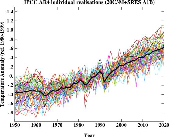
It shows the earth annual average surface temperature for each of 55 (56?) runs. I suspect these are all A1B runs.
I told Pete B this is a little deceptive because you can’t see the clustering by models. So, I created a slightly different graph. I did the 25 month average (because I already had the model mean coded that way.) Then, instead of assigning a different color to each run, I assigned a color for each *model*.
Here you can see that spread of the runs doesn’t really “weather” or “internal variability”. At least part of the spread is due to the mean for each model being different. This happens because different models have different climate sensitivities (and different ocean heat uptakes and so on.)
So, yes, I mean different models have different sensitivities.
Lucia,
That last graphic is very nice. One thing I note is that there is more (and ever growing) spread after 2001, and relatively less spread pre-2001.
.
For those models with multiple runs, would it not make sense to show which are clearly beyond the pale? I mean, if the divergence of some models from reality is statistically significant at high confidence, then why not throw out the bad apples and consider the average and range of projections for only models which remain (individually) plausibly accurate? Sort of a ‘plausibly accurate IPCC projection range’? It is the sort of thing I would expect folks like Gavin to do, but I am guessing he never will.
Nyq,
An explanation is a statement that points to causes. A model by itself doesn’t point to anything. That would require context which is outside the model.
Andrew
SteveF
This is caused by baselining. The mean temperature from 1980-1999 was mathemagically set to 0 for all runs. Consequently, the spread during the period is constrained. If all models were “true” in the sense of getting the correct model mean at all times (t), the spread would remain the same over all time. However, if individual models have different trends, the spread in runs will diverge because the contribution of the different mean trends adds to the effect of internal variability. (If I showed regions before 1980, you’d see larger variability during that period too.)
Yep. 🙂
RE:steven mosher (Comment #76203)
“As we know the gases in the atmosphere control the rate at which radiation escapes back to space. Adding more GHGs to the atmosphere will result in a warmer planet. The questions are.
1. How much warming over what period of time.
2. How accurately do we know this
3. what, IF ANYTHING, can we do or should we do to change this.”
I like you fuel mileage computer model analogy and agree with you conclusions. Allow me to introduce you to a little climate change gremlin:
http://www.wired.com/images_blogs/photos/uncategorized/2008/04/18/solarflare.jpg
@ivp0, the sun, if anything, is less active now, and any forcing it is producing is a cooling one.
PeteB:
I think some of them clearly are “going astray”:
Look for example at the IPCC review of model ENSO predictions.
Seriously, that some models will break down shouldn’t be a surprise. They use different model assumptions and forcings in general, some of these have to be wrong.
RE:bugs (Comment #76223) May 23rd, 2011 at 7:48 pm
“@ivp0, the sun, if anything, is less active now, and any forcing it is producing is a cooling one.”
You are so absolutely right Bugs! Kinda consistent with that downward trend over the last 10 years in the OP. Quiet sun, downward trend… hmmmm.
Carrick, Yes, you are right, I didn’t quote Bill properly, what Bill said was
All I am saying is these run’s aren’t necessarily going astray, just in the shortish term. in some cases the weather noise is masking the trend, in some cases the weather noise is exaggerating the trend over the shortish term. Once you get to 15-20 years, this effect will be a lot smaller.
The larger point I was making was that it can be slightly misleading to compare something that includes ‘weather’ noise – the observations, with something where the ‘weather’ noise has, to some extent, been averaged out (average of model runs)
That’s a great graph
That would be good news !
Re PeteB:
If you look at the difference between the multi-model mean and observations to get an estimate of “weather variation”, removing the ENSO component from observations as the primary source of this variation, from 1975 to ~2001 you can model the remaining noise as a small white component:
http://troyca.files.wordpress.com/2011/05/mmmandhadcrutninoadjusted.png
More details at (http://troyca.wordpress.com/2011/05/23/comparing-nino-adjusted-hadcrut-to-cmip3-a1b-mmm-projections/)
Of course, once you switch from hindcast to projections, the models go off the rails. If we’re to believe the MMM represents the true underlying forced component, then either the non-ENSO weather noise is actually quite small (and consequently the larger errors pre-1975 are the result of less accurate forcing and temperature data), or our universe’s realization of 1975-2000 experienced very little weather relative to all possible realizations. The former would mean that weather noise can’t explain the difference in the 2001-2010 trends.
Granted, the inaccuracy in some of the forcings projections might be the cause of part of the divergence (solar was mentioned above), but for reasons mentioned by others, it’s not likely to be fully responsible.
Lucia, Just looking again at that graph, am I right in thinking that some models look as if they have much more variance between runs than others, or is it just that some models have many more runs included ?
All the runs for the orangegy brown model are quite close (and too high), wheras the different runs for the pinky purple seem to be very variable
Andrew_KY (Comment #76218) “A model by itself doesn’t point to anything.”
We are probably using the term differently. I’d assume a mathematical model includes a particular interpetation of its terms. That would be consistent with the formal logic usage of the term ‘model’. So, for example, f=ma isn’t a model – it is just an equation – but if we say f is voltage and m is resitance and a is current (in some appropriate units) then we have a model. If we say f is force and m is mass and a is acceleration then we have a very different model.
Re: Andrew_KY (May 23 12:54),
Climate is long range stats. So, you are wrong I do understand climate.
And yes models are explanations.
D= R*T. The distance I travel can be explained by this mathematical model.
########
Andrew. I think you dont know what models are.
PeteB-
It’s the former. Some models have an amazing amount of noise and at quite short time scales. Some have very little. You’d see the amazing noise even more clearly if multiple very noisy models didn’t happen to be assigned colors that are very close in value. (i.e. red/magenta/violet.)
Applying tests to the noise shows the standard deviation of 10 year trends is different from model to model. So the internal variability of climate is different from model to model.
Steven Mosher,
If you think climate is numbers, you clearly do not understand what climate is.
Andrew
Lucia,
Yup. The magnitude and spectrum of variation in any accurate model ought to match the historical record reasonably well, while also matching the longer term trend. Any model which is grossly different from the historical record in variation must have substantial internal misrepresentations of the real climate; the uniform failure to duplicate the pattern of ENSO is the most obvious case. What troubles me about treating model projections of ultimate sensitivity to forcing as credible, in terms of public policy, is that the models so consistently fail to match the real climate in multiple important aspects not just overall warming. The obvious kludge of using whatever aerosol history best matches the historical temperature trend only makes the structure of model variation even more important in evaluating model accuracy (since aerosols are adjusted to give match the historical trend, no matter how far off the model may be).
.
As I think I have noted before, when the next round of model projections is published (AR5) it seems to me likely that a lot of arm waving will be included about how those old models from AR3 and AR4 were bad, but now the new and improved AR5 model projections are sure to be right (and we must of course stop burning fossil fuels immediately!). I find this whole process so intellectually corrupt as to be laughable, save for the huge economic damage that could come from it.
Andrew_KY (Comment #76239) “If you think climate is numbers, you clearly do not understand what climate is.”
Which is like saying that somebody who thinks a map is accurate believes that terrain is paper.
Nyq, Quoth Steven Mosher: “Climate is long range stats.”
Please give me your translation of that sentence, since evidently you read unfamiliar meanings into words I thought I knew.
Andrew
@Andrew_KY (Comment #76269)
Here’s a definition of climate:
– The meteorological conditions, including temperature, precipitation, and wind, that characteristically prevail in a particular region.
.
If you leave out the “characteristically prevail” part it is a definition of weather. If you watch the weather forecasts you’ll notice that temperature, precipitation, and wind are often described using numbers (25C, 2mm rain, 10 m/s wind speed). Is that a problem for you?
.
Tell us how you would describe and track changes in the meteorological conditions that characteristically prevail in a region (climate) in any detail without letting these typical meteorological conditions that we call climate be represented by numbers or “long range stats”.
Niels,
No, and as scientifically as possible.
Sherlock mosher still made an incorrect statement.
Andrew
Mosher,
Glad I ventured back here and find the conversation continuing. First, thanks Mosher for a thoughtful response. I enjoyed some of your analogies. Yes, I know there are 22 models or more. In my post above I left out a captical C in referring to some of those models that assume high climate sensitivity to CO2. I wrote “Yes, temperature data can not “disconfirm†or invalidate the IPCC and Hansen hypotheses (models) in the short run. However, we can say with confidence that the temperature data of the last 13+ years does not support those AGW models or even AGW models.” It should read “or CAGW models.” Yes, this is shorthand. I realize there are no AGW or CAGW models as such. I’m referring, of course, to the inference that many journalists and politicians make- with little pushback by mainstream scientists who know better- that 1) models are some kind of evidence and that 2) models are predictions and 3) that models which project very significant warming (say more than 3 degrees C per century which I refer to as CAGW models) have some historical empirical support from the temperature data. Britain and Australia right now are making very expensive politicalm bets based on catastrophic global warming that is not happening. You would never know it’s not happening by reading/watching 90% of the MSM. We had 20 years of significant warming. Now we’ve had 13+ years of flat lining temps. Before the 20 years of significant warming, we had 30 years of slight cooling- the ups and downs to which you refer. The temperature data is inconclusive; the recent 13 years of flat lining is not a danger sign that we must act immediately to reduce CO2 emissions. The temperature trend of the last 33 years does not portend CAGW. The temperature trend of the last 63 years is pretty close to the best estimates of the previous 65 or 165 years. Where’s the beef?! The sea level trend has recently fallen back to the several hundred year average, as best we can tell. So you suggest we need to assume, as primary, the forcing we understand best, GHG, even though we don’t understand the feedbacks which makes all the diffrerence. Despite the alarmism which dominates British and Australian politics and the MSM headlines, there’s nothing alarming happening. Thye most alarming thing happening is that scientists, including you, do not acknowledge this.
SteveF (Comment #76241)
May 24th, 2011 at 8:00 am
Seconded!
Steven Mosher said,
“Simply, the observations tell us that some models are better than others. That’s not surprising.”
At what point can we say with some confidence that models x and y are the most reliable and attempt to narrow the projected impact to a workable range?
A few people that have standing in the climate science community have mentioned that the range of sensitivity should be lowered. And there are plenty of idiots like me that see that 2.1 to 2.7 is likely the upper limit.
SteveF,
The ocean lag is interesting. It would seem to me that most of the impact of thermal inertia would be shorter term, 1 to 2 years, with a much smaller impact from greater than 5 year lag. The only place I see a significant long term lag impact is early in the OHC data when it is basically… caca. The more recent data, which I assume to be better, correlates pretty well with a 10 moving average of surface temp (using just the satellite era data). Is there a better way to estimate the buffering effect of OHC lag on estimated surface temperature?
Andrew_KY (Comment #76269) May 24th, 2011 at 2:01 pm
‘Nyq, Quoth Steven Mosher: “Climate is long range stats.â€
Please give me your translation of that sentence, since evidently you read unfamiliar meanings into words I thought I knew.’
Cool – I’m the prophet of Mosher now! Well he would appear to be saying that while weather is short range stats, climate is long range stats. He is using what is know as FIGURATIVE language. http://en.wikipedia.org/wiki/Figurative_language
For example if you said to somebody “what’s the weather today?” and they answered “27 degrees and 30% chance of rain” it would not be normally deemed socially acceptable to then criticise your correspondent because they had given you statistics instead of the weather.
Is the climate LITERALLY long range statistics. No. Is my height literally 1.89 metres? No, it is the vertical extent of my body when I’m standing. No wait, that was a bunch of words were as my height isn’t a bunch of words it is an actual physical property of me. Arrghh more words!
ANyway perception, words, intelligence metaphors etc etc – assume I just keep rattling on like that for awhile. Hmm no good? You’re right. I did promise ACTION in an earlier message.
So even as I continue to witter on like some undergraduate who has just read a philosphy text for the first time, you notice that creeping up behind me is ninja, clad all in black. In his hand a razor sharp dagger poised to cut effortlessly into my spine. Your eyes grow wide in horror – you would cry out a warning but my sophomoric ramblings about the limits of the noumenon have actually destroyed your ability to articulate even rudimentary speech. Yet just in time the very gleam from the ninja’s sword is reflected in your eye. I turn just in time to avoid the deadly arc of the ninja’s blow.
With a characteristic wooshing noise I transform into samurai robot (available as a package from your nearest CRAN mirror) and blast the ninja with both missile fflanges….
…but they past straight through him!
This was no ordinary ninja but a GHOST ninja! Conjoured up by a climate model projection gone awry!
It seems, once again, that the prediction of extereme weather events has been taken too literally by a computer overlords and they have included deadly ghost ninja assasins in the panolpy of potential disasters awaiting us!
Luckily you still have a baseball bat – as yet unconfiscated by the forces of leftiness (who curiously have overlooked my ability to turn into a missile firing samuria transformer robot)….
“Eat bat!” you cry swining at the black glad ghostly figure….
You should dance your answer, Nyq. After all it offers a more proximal description than mere language. Unless… unless you could just be the weather or climate. That would be the best description of all. Just be it.
“He is using what is know as FIGURATIVE language.”
Nyq, Yes, Steven Mosher is the Poet Laureate of Global Warming. He doth spin fanciful tales to horrify and delight, weaving the tapestry that is your imagination.
Andrew
Mark (Comment #76330) May 26th, 2011 at 5:45 am “You should dance your answer, Nyq. After all it offers a more proximal description than mere language. Unless… unless you could just be the weather or climate. That would be the best description of all. Just be it.”
My next post will be a jazz solo on a theremin. The difference between weather and climate will be represented by pauses of silence and the rustle of the audience’s expectations.
“Nyq, Yes, Steven Mosher is the Poet Laureate of Global Warming.”
Bingo – figurative language and irony (or at least sarcasm). I, the reader, know that you are not LITERALLY claiming that Steven Mosher has been appointed Poet Laureate or even that “Global Warming” has its own poet laureate.
Having said that his use of iambic pentameter in the Crutape Letters was a bit forced. eg Page 14
“You are about to en-ter a world where,
poe-ple in white lab coats do not play fair,
not with facts nor with fig-ures and certain-,
-ly not with each oth-er forsooth begad.”
Dallas (Comment #76284),
Yes, the ocean lag is interesting, but for sure complicated. The thermal mass of the surface layer (averaging about 55-60 meters depth globally) is sufficient to (by itself) add considerable lag to the temperature response to a change in forcing (eg, several years approach constant for a modest size step change). The problem is how the surface layer transfers heat to the thermocline. If the rate of heat transfer down the thermocline is relatively fast (suggesting a large continuing heat loss from the surface) then this implys relatively higher sensitivity. If the rate of heat transfer down the thermocline is very slow, then this implies small heat loss and relatively lower climate sensitivity.
.
There is not a single approach constant, but a wide range of approach constants, from a few years to multiple hundreds of years. But if the current overall rate of heat loss down the thermocline is known via measurement to be small, then we can safely conclude that the currently measured response to a forcing is not too far from the ultimate response. That leaves aerosols as the primary source of uncertainty in climate sensitivity.