In comments Ed Barbar wrote
Provided that the noise is random over time and provided the screening time period is different than the time period used to determine the “m†in w=mT+b, it seems there should be no added bias. Yes, you might exclude some perfectly good trees, and include some bad ones, but the noise will tend to cancel and not bias “m†in any particular direction.
You will see I agreed, and then Carrick agreed with one caveat:
Lucia hit on this a bit, but for temperature proxies, the noise is highly correlated. So you’d need to widely separate the period where you’re correlating to and the period where you’re computing m. Otherwise, I agree with your comment too.
I hadn’t thought of the need for separation, but immediately agreed Carrick was correct about that. I will tentatively suggest that if the ‘noise’ is red, we can estimate the required gap between the ‘screening’ period and the ‘calibration’ period as being exp(0.1)/exp(R1) intervals where R1 is the lag 1 correlation coefficient for your time series. This interval reduced the correlation between the closest points in the two periods to 10%. More refined calculations would be possible if one stated some more specific requirement. Note that using this rule, if the lag 1 correlation for noise was 0.9, you would need a gap of roughly 22 measurement points between the period during which you screened and the one in which you computed the calibration (m) that permitted you to back out the best estimate of the temperature from something like ‘ring widths.
Continuuing with the same general idea of examining hypothetical effects using synthetic data, a sinusoidal temperature as the “truth” we wish to detect from our proxies (i.e. ‘treenometers’) I’ll compare results where:
- The ‘proxies’ consist of 1000 ‘treenometers’ with R=0.25 relative to the true temperature plus 1000 ‘not-treenometers’. So it’s a case one might imagine would benefit from screening.
- The “noise” in each treenometer has a lag 1 autocorrelation of R1=0.9. This differs from previous examples which all had R1=0. I introduced this to permit discussion of the point Carrick made. Note that having a large lag 1 autocorrelation aggravates the bias introduced by screening.
- In one case I will both screen and calibrate during the same period. This is the method that introduced bias that we’ve all been seeing. In the second case, I will screen during the final uptick but calibrate during a much earlier period. This method will be seen to be unbiased– provided we ignore the information from the proxy reconstruction from the ‘screening’ period and for a period just prior to the ‘screening’ period. (Ignoring information during the screening period is fine because we do have data during that period.)
Biased case: Screening and Calibration period identical

Above, the screening period is shown with vertical black lines; the calibration period is shown with vertical dashed blue lines; these overlap.
Notice that in this case, the green trace which represents what an analyst using this method would report as the estimate of temperature in the past is severely biased. In particular, the peaks and valleys are squashed. If the analyst was unaware that screening did this, they would conclude the reconstruction shows that current temperatures exceed those that occurred in the past — and by a humongonourmouse amount. (Mine you: I am picking my parameters to make the biases visible. The magnitude of the potential bias in any paper will depend on the properties of their treenometer and the details of what the analysis did. But this does show what screening tends to do. If you screen, you should estimate the magnitude of this effect on your results. Better yet, avoid methods that introduce this problem.)
Unbiased: Wide separation between Screening and Calibration period
Following Ed Barbers very good suggestion, I performed the calibration.

Above, the screening period is shown with vertical black lines; the calibration period is shown with vertical dashed blue lines. Based on my rule of thumb described above, for an lag 1 correlation coefficient in the noise of R1=0.9 to avoid appreciable bias the calibration period in which we compute ‘m’ relating tree ring width to temperature should be separated from the edge of the screening period by roughly 22 years. This means my calibration period should be outside the region indicated by the red line. Note, I separated the two by nearly twice that required amount.
When viewing the reconstruction, we now see that for all ‘years’ prior to the one marked by the red line, the screened and unscreened reconstructions match each other and also match the ‘true’ temperature rather well. There is no visible bias. However, after the red line, the screened reconstruction (green) is biased relative to the ‘true’ temperature. But this bias is ok provided we simply ignore information from the screened reconstruction during the ‘screening’ period and the 22 year buffer period prior to the buffer period. Once we do that, we could compare the reconstruction in the past to current temperatures. Both reconstructions would give us the correct result: The temperature in the current period is not an all time record (in this toy problem.)
So, it is possible to use screened data. However, when doing so one must first recognize that screening can introduced bias and select subsequent procedures to avoid introducing that bias.
What’s next
I keep promising that I will show a case where screening can reduce errors in the reconstruction. And later I’ll talk about how we might further improve screening by examining the distribution of the correlation coefficients to identify the ‘not treenometer’ in the batch without simultaneously removing the ‘treenometer’ that contain a signal, but had low correlation coefficients with temperature during the screening period. I promised that earlier, but Ed’s suggestion was a good one, and so I wanted to show it.
Of course: In true climate -blog Gergis fashion, I will claim that I thought of Ed’s suggestion before he mentioned it in comments. But I hadn’t done it, or mentioned it etc. And, in fact, I did in a sort of casual way while doing something like mowing the lawn or exercising at the gym. And then all of you can decide whether you believe I thought of it– just as you can all decide whether those who claim to have thought of such things before the first person who was brave enough to suggest the idea did so in public.
In this case, the person who seems to have suggested this in public first seems to have been Ed. So, I think he deserves credit. (After all, even if I did think of this before he did, if he hadn’t mentioned it, I might have forgetton the idea anyway. That’s what happens to lots of ideas I get while mowing the lawn.)
So you have demonstrated that you can avoid a calibration bias by screening and calibrating independently. It doesn’t appear that the screening had much of a beneficial impact in this case. What is the distribution of good/not-good in the screen output here?
Actually, if you squint hard, there is a very slight benefit to screening here. The unscreened line contains a little more noise and because the noise is red, that noise results in mis-estimating the ±95% range of temperatures in the proxy reconstruction.
To see this, look at the violet and green horizontal lines at the top of the oscillations. Notice the green peaks on avearge match “real” (black dashed) a little better.
I can discuss distributions of what was screened out vs. what was retained later. But for now, this is a fairly powerful method to improve the screening. It’s also easy. So I thought it was better to show this than to discuss the ‘tweaks’ you might do to improve the screening beyond this.
I think it might also make people whose inclination is to believe that screening by correlation must work be willing to see that it is biased if you do it wrong (that is– by screening by correlation and calibrating in overlapping regions.)
How do you estimate the chance that you are just (un)lucky with the proxy and the correlation with temperature is just due to chance?
I had a look at the Gergis proxies and here are the R Squared correlations with HadCRU based on end year. There are 437 different starting dates for the 71 year (1920-1990) calibration line-shape.
The end year of 1990 is not always the best by any stretch of the imagination.
http://i179.photobucket.com/albums/w318/DocMartyn/RsquaredofProxiesvsHadCRU.jpg
We can’t do this with you ‘toy’ sine waves, but can we do it on real proxies?
Doc–
For the toy problems, I’m currently just throwing away 56%. I’ll talk about how one might better screen later.
But I think the a better question might be “How do you estimate whether a negative correlation was sufficiently low to justify assuming a tree (or series) contains no temperature signal?”
Remember: All these trees (or proxies) were initially included because someone suspected the should have or might contain signals. They did not just pull out every possible time series for every possible thing in the world going back 400 years and sift. They 67 proxies were examined because someone thought they might (or would) be correlated with temperature.
Lucia, I mentioned in an earlier thread that there look to be discontinuities in the Gergis proxies and that when corrected seems to remove nearly all of the autocorrelation. Status of stationarity needs to be determined before autocorrelation can be calculated. I haven’t had time to delve further unfortunately.
Agreed. The reason I use toy problems is to illustrate the qualitative effect a a particular analytical choice without worry about additional issues that might inject additional uncertainty.
‘lucia
But I think the a better question might be “How do you estimate whether a negative correlation was sufficiently low to justify assuming a tree (or series) contains no temperature signal?‒
That is indeed a much better question and one to ponder.
(*smiling) How long till one applies this method to actual tree data?
MDR–
Do you mean me? Or someone else? I may never apply it because that’s not the main point in showing the potential biases. The purpose in showing biases that arise from screening is:
1) To show they really do exist.
2) To show some circumstances in which they exist and so
3) be able to explain why people who do screen based on correlation need to either fix their method to avoid the bias or estimate the uncertainty introduced by screening when interpreting their data. The latter would involve a) doing a rather complicated calculation to estimate the magnitude of the biase and correct and estimating the uncertainty in their correction and showing the new larger uncertainty on their graphs.
We can get a defensible answer to that question. Of course, since it’s statistics we need to make assumptions. But it can be done.
Lucia:
I think this is a good approach. Again using the spectral method you can get away from strictly red-noise.
If I had to pull a number from my hat (this is a SWAG), use 30 years.
Very nice demonstration.
Sean:
Lucia’s addressed this, but this case was constructed to verify that you don’t introduce bias using Ed Barbar’s method not to demonstrate the putative advantages of screening.
Now you can go back and throw in a certain percentage of “non-temperture proxies” and see how robust your technique is against this.
Lucia,
Very nice.. and I do think Ed came up with the idea first.
.
But what happens when 60% or more of the trees really contain no information at any given point in time about temperature (just reddened noise, no temperature information)? And more importantly, what happens if the specific individual trees which carry temperature information (however noisy that might be) changes over time? (eg. divergence)
.
I don’t think correlation based selection can ever be valid except when the assumption that all the trees respond to temperature is correct. But even if the trees don’t satisfy that assumption, using all the data will generate a valid reconstruction every time.
SteveF–
In my example, 50% of the original sample contain no information about temperature at all. the other 50% contain information — but each is noisy.
Well…. everything goes to heck!
Having some trees that don’t respond to temperature can be ok– provided your screening method doesn’t make it seem like they are responding .
Its usually safer. The analyst is much less likely to trick themselves.
There are at least hypothetical circumstances where screening could be justified. Similarly, even in a lab, there are circumstances where the diagnose a data point as being a contaminated outlier and throw it out.
For example, with LDV, we know that most velocity measurements are from light scattered by a particle passing through a sampling areas. But some “measurements” will be shot noise that happens from time to time. The shot noise will frequently appear to exceed the speed of sound or be many, many, many, many standard deviations outside the spread of all the other data. Say you take 10^4 data points and 1 point is 20 sd’s out there. There are rules you can invoke to justify pitching that data point out. There are things you can do to persuade people it’s ok to pitch some data– and yes, you are doing it based on the data itself.
We could do similar thigns with the population of correlation. The problem is: It’s harder because correlation goes between -1 and 1. But, at least hypothetically there are justifiable ways an analyst could either throw out a tree or — more likely– a stand of trees even under the assumption that individual trees (or stand of trees) response to temperature is invariant over millenia and the behavior during the screening (and calibration) period is typical.
My favorite from my work days was: That result is wrong, run it again. Too which I had several responses, the first of which was: If you already knew the answer, why did you bother to submit a sample? The next was: Submit another sample and I’ll run that, but I won’t analyze another aliquot of the same sample.
When control charting, if you get an out of control data point, you absolutely need to know why that point is outside the range. There are lots of possibilities starting with the process actually being out of control. But you may have underestimated the process variability or there may actually have been a problem with the measurement, contamination during sampling, calibration drift, etc. But the one thing you can’t do is make measurements until you get one that is inside the control limits and use that instead of the out of control point.
Lucia,
Thanks.
Throwing out clear outliers is justifiable under a lot of circumstances, of course, but you usually have solid arguments (like a data point 20 SD from the mean almost certainly isn’t right!) when you do that.
.
What I guess rubs me the wrong way is wading into a cesspool of data and declaring some valid and some not, even though you have absolutely no idea why. It is the lack of understanding of root causes which suggests the entire enterprise is highly doubtful. “CINC” (correlation is not causation)
DeWitt Payne (Comment #98543),
I have essentially identical experience; improper data rejection is rampant across a wide range of industries. It is easier to just run another test than piss off the boss with an out-of-control data point. It is (of course) almost always the boss who is at fault for making the generation of correct (but bad) results have negative consequences.
Another example.
In looking at Icoads data we have the ships location over time.
When the change in location indicates a ship travelling at 1000 knots well, we know something is amiss.
Similarly, when the most influential tree in the world shows 6 sigma growth and plant biologists tell us that’s not physically possible, well we would remove such a tree. Unless, of course, we liked the fact that it corellated well with temperature.
Opps.
SteveF
That rubs me the wrong way. But also, using what amount to self contradictory assumptions or procedures that just don’t work.
Also: not admitting that you just can’t “fish”. The problem with some of the correlation screeing is it resembles fishing a lot more than identifying and tossing outliers from data that collected (or even selected) based on what were considered valid criteria. If you want your results to have a decent connection to reality, if you collect (or select) data based one what you consider valid criteria, afterwards, if you are going to screen for outliers, you test to see if you can prove it’s inconsistent with the hypothesis that it contains a signal.
In the case of somethign like Gergis, if the 67 proxies they started with were chosen because someone thought there was a good reason to expect them to be correlated with temperature, they shouldn’t throw any away unless it is so strongly negative that it is not consistent with containing a signal. In fact– if they were going to screen on R, they should have
*) Under some statistical model for the noise (which would have to be justified based on the data) find the distribution of Rs they would expect a population that was pure noise. (This is easy for white noise. For R computed based on 100 data points in the time series, you expect to get roughly 95% of the data with R’s between t=0.196 and -0.196).
2) Now, since initially they chose these because they expect them to contain signal, and throwing ways anything with a value of R that is even a tiny bit over 0 causes bias without reduding noise, the want to only throw those they are nearly certain are ‘noise’. So, in the first place, that means they should only throw away thigns with R<-0.196. But…
because they have 67 data, even if something is just borderline, they should expect have about 3 or 4 data with R outside the range ±0.196. So, to decide what to pick, they might find the t value associated with something much stricter!
But at least they shouldn’t have thrown anything out unless Rmin was less than -0.196. But instead, they turned this on it’s head and required each to “prove” itself. So, what they did was equivalent to requiring it to be greater that 0.196. That’s nuts!
The latter is the sort of thing you might do if you are doing in the first step of some sort of exploratory data mining. Wallmart might do that if they were fishing to figure out what factors caused people to buy ice cream or something. (Then later, you– or Wallmart– would do a repeat experiment with truly out of sample data to figure out if the stuff you fished for was real.)
Can this method really work though?
“provided the screening time period is different than the time period used to determine the “m†in w=mT+b”
I’ve said this over and over, to little effect, but the point of Gergis’ screening is to make sure she can determine m. If she can’t, she can’t use the proxy. As in can’t.
So screening on another period may have some other virtue, but doesn’t do the job. And it’s not clear what job it does do.
In practice, there aren’t spare periods available. You need every bit of overlap time for calibration and verification. And having a gap just makes it worse.
I have said that there is a real screening fallacy. You lose independence of the information in the screening period. That’s still a problem here.
Yes. This you really have said over and over. And they way she does this is wrong.
I am unaware of your having brought up the notion of using different time period.
Uh… so you are saying this process doesn’t do the job?. But also claiming you’ve said it does to the job over and over? And you are saying both those clearly contradictory things in adjacent paragraphs?! You’ve out done yourself.
But in any case, it’s little surprise that people don’t understand what point you think you are making.
Screening on a different period from the calibration does “do the job” if “the job” is to try to “fish” for the “true treenometers” without biasing your estimate of temperature in the proxy reconstruction. It may not be the best way to do it, but it does do that job.
I realize this is why people might prefer finding a different way. But calibrating and screeing in the same or overlapping periods will result in a reconstruction that is biased relative to reality.
You’ll have to elaborate what you mean by “lose independence of information” and clue me in on what the problem is here. But because if you’ve said this somewhere, I don’t know where that is, I have no idea how to use my googlefoo to find your discussion and anyway, I don’t plan to have spend a lot of time using my google-foo when you could just explain what you mean.
I’m perfectly willing to believe that even if we do what I did above which solve one problem others still remain.
Nick, what do you think of the R2 values for fitting the 1920-1990 calibration period over the range of data?
http://i179.photobucket.com/albums/w318/DocMartyn/RsquaredofProxiesvsHadCRU.jpg
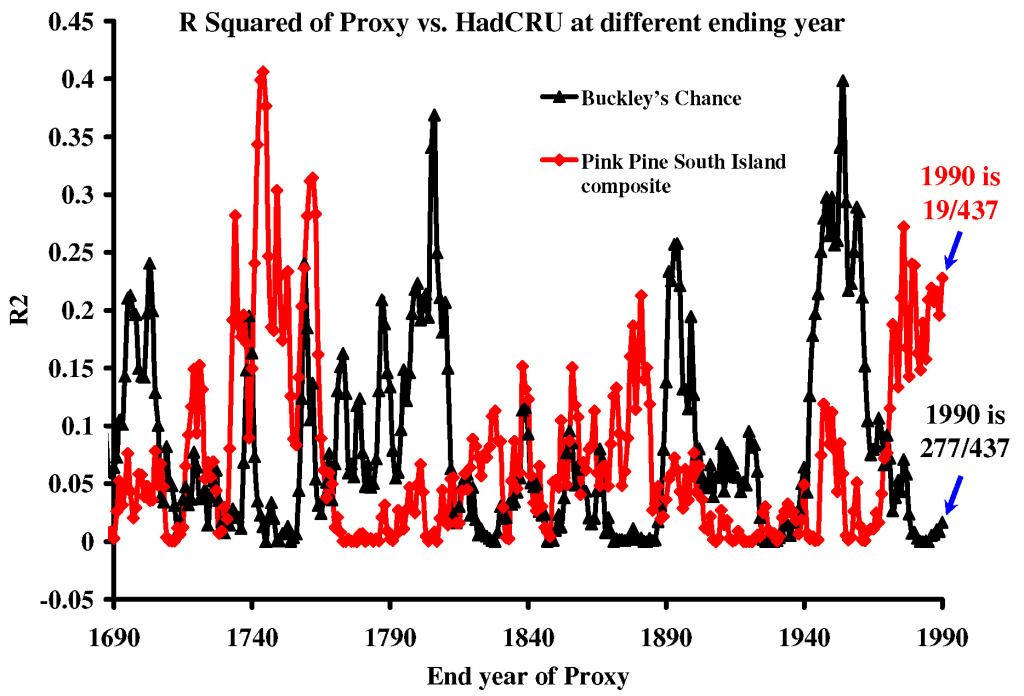
It is quite clear that previous periods of growth in the proxies are a better match for the ‘unprecedented’ warming of the modern era.
Why can’t I see a drop in temperature following Mount Tambora (1815) or Krakatoa (1883) ?
Now call me Dr. Stupid here, but I would have thought the majority of data sets should respond to events in the Southern Hemisphere that resulted in cooling of the Northern Hemisphere. Why can’t I see a 1+ SD event following the Mount Tambora or Krakatoa in any of these wonderful temperature proxies?
Come on Nick, explain for once.
Doc–
Could you explain how you define “R2” for your proxies? In words or algebra. Because I don’t know what that is supposed to mean.
Lucia,
“And you are saying both those clearly contradictory things in adjacent paragraphs?!”
They are not contradictory at all. Gergis actually (in effect) calculates m. Significant values she can use and proceeds. Others she can’t. Screening on a diferent period wouldn’t help that.
But any method will, one way or another, be unable to use a proxy that doesn’t have some observable relation to temperature. There’s no sensible arithmetic you can do. In a PCA method, for example, the proxy will be near orthogonal to the retained eigenvalues. Whether you drop it in advance or not, it will have no influence. That was my earlier point about screening and weighting being little different.
“You’ll have to elaborate what you mean by “lose independence of information†and clue me in on what the problem is here. But because if you’ve said this somewhere, I don’t know where that is,”
It was in my first comment here on the topic. And in my first comment at CA, where it was deemed too obtuse to respond to. But it’s obvious. If you screen on concordance with temperature, you’ll get concordance with temperature in that period. That’s not independent information.
Sorry Lucia, I used the RSQ function in Excel which is the square of the Pearson correlation coefficient through data points of HadCRU 1920-1990 vs the proxies in 71 year blocks.
Doc,
About R2, what Lucia said.
On volcanoes, I earlier linked this paper on the topic.
“Nick,
It was in my first comment here on the topic.
If you screen on concordance with temperature, you’ll get concordance with temperature in that period. That’s not independent information.”
Are you saying that one gets information in the pre-secreened period about line-shape, BUT, that this cannot be calibrated using the relationship between line shape and temperature in the screening period?
Nick, answer the SPECIFIC question. Why can we not observe a large drop, the multi-year recovery in any of the temperature proxies for the two largest volcanic eruptions in the last 1,500 years?
Don’t link to a paper that is speculative bollocks; explaining why your thermometers don’t respond to a temperature signal due to ‘the effects of diffuse radiation’ is just displacement activity.
O.K. So now your trees respond to temperature, water, fertilizer, all changes in the local biosphere and to changes in ‘diffuse radiation’.
Very good.
So corals respond to the sonic booms generated by volcanoes in a manner that exactly the same size as the changes in temperature, but of a different sign. 18O suddenly change their fractionation properties due to dust.
In fact, all proxies ignore volcanic cooling events, but faithfully respond to all other cooling events.
Doc,
No, I’m saying that when you calibrate, you sacrifice independence; it’s part of the deal. Suppose I have five thermometers, and I want to get a very good measure of temp in a room. Then I might take five readings, and maybe I can learn more than I would from one.
But suppose I believe that one of those thermometers is more reliable and calibrate the others to it. Then I might have four better thermometers for other purposes. But there’s no point any more in using them all to measure the temp in the room.
My CA comment on this linked above is here.
Nonesense. We know that because the time periods are short, her computed ‘m’s are biased high relative to the real average value of ‘m’ for the batch she kept. And the reason they are biased high is that she hasn’t merely thrown away bad proxies, she’s kept some bad ones that were accidentally good and thrown away good ones whose noise made them look bad in that period.
If she wants to get an unbiased estimate of the true value of “m” for proxies she screened, she needs to use a different period.
Of course not. But that doesn’t mean you can screen out and then compute ‘m’ using the period you used to screen. It doesn’t work.
Doc,
“Nick, answer the SPECIFIC question.”
Sorry, I don’t have answers for everything. As that paper says, it seems to be a puzzle.
If you want a good measure of temperature in a room use one thermometer calibrated to a known standard within its certified range of operation. You will then be able to quote temperature within a known tolerance. Belief has nothing to do with it.
http://www.npl.co.uk/publications/guides/comment/comment-temperature-guide
Nick–
I’ve looked at both comment you link and you are being obtuse in both.
As for this
This is just stooooopid. Almost unbelievably stooopid (but I’ve know other stoooopid people who have concocted similarly stooooopid idea.)
You calibrate the thermometers in an external calibration. You don’t calibrate them using data from the experiment you are measuring.
If you external calibration says one thermometer is good and the others don’t work, then you can use that.
Lucia,
“But that doesn’t mean you can screen out and then compute ‘m’ using the period you used to screen.”
I’m not sure we aren’t saying the same thing here. What I’m saying is that having in effect fitted m to match the observed temp, it isn’t meaningful extra information about the gradient in that period.
“If she wants to get an unbiased estimate of the true value of “m†for proxies”
But she’s not. She’s trying to calibrate, which is quite different. She needs a best estimate of m for each proxy alone.
Lucia,
“You calibrate the thermometers in an external calibration. You don’t calibrate them using data from the experiment you are measuring. “
Where did I say anything about using data from an experiment? All I’m saying is that you have five scaled thermometers. If you have one that you believe is more accurately scaled, you can calibrate the others to it.
But OK, a more homely example. You have five clocks. The time was set a long time ago and has wandered. You check them all and get some sort of average when you need.
But suppose you believe one has held its time better. So you set the others to match. Reasonable, but you’ve in effect put all your faith in one clock. The others don’t give you independent information.
Doc–
So…. it’s the correlation coefficient between Hadcrut and a proxy computed over 71 years– but then sliding? So is the year shown in your axis the final year? I still don’t know what you are doing. HadCrut is from 1920-1990. Are you saying that for some reason, you took a proxy from say, 1640-1710 and computed the RSQ with HadCrut from 1920-1990? Why? What’s that supposed to tell us?
First: This isn’t remotely what Gergis did.
Second: This doesn’t improve your estimate of the time.
Third: You con’t claim it improved your estimate of the time.
Fourt: I have no idea what you plan to do with these clocks later. But it’s hard for me to imagine a experimentalist who thought this was “reasonable” in most experiments where you needed an objective measure of time.
Nick
First, she’s trying to calibrate her method of figuring out the temperature from the ring widths. To obtain a good calibration, she needs an estimate unbiased estimate of the true value of ‘m’. She will get a better one by computed the ‘m’ over a period that differs from her screening period.
If you would finish your thoughts and to connect “she’s trying to get a calibration” to include “she’s trying to get a calibration to determine Y based on X” you might be able to unbefuddle yourself. When you calibrate, you want a calibration that can be used to obtain an unbiased estimate of Y based on X. For Gergish’s method getting a bunch of ‘m’ cherry picked to keep those that are higher than the correct value and tossing out those that are lower than the correct value is not a good way to get a calibration. It’s bunk!
“lucia
Are you saying that for some reason, you took a proxy from say, 1640-1710 and computed the RSQ with HadCrut from 1920-1990?
Yes
“Why? What’s that supposed to tell us?”
The conclusion was that the modern period was unprecedented, which I take to mean that it has never happened before.
Now if the correlation with the fastest ever temperature rise gives one a better fit to the a proxy some 500 years ago then it means a number of things, such as
1) Such temperature rises have happened, many times, in that local in the past.
2) The proxy may not be responding to temperature.
3) You cannot average proxies in the per-calibration period because some have seen seen big rises in some periods and other have not. Such heterogeneity means that a huge number of proxies need to be acquired.
Doc, It would be fun to reverse all the proxies 🙂 Isn’t there a satirical journal Nurture or Neuter to publish in?
Doc–
I honestly have no idea what we learn from your graph.
Nick:
You sound more and more like Claes every day. I know you really didn’t want to hear that. 😉
My theory is this is some cognitive disorder that numericists develop from writing too many Runge-Kutta routines where they suddenly have an “ah ha!” moment and think, even though they’ve never taken any data, they are now experts at measurement theory. /stinker
Whether your statement is true depends whether all of your clocks have the same temporal resolution—-
Suppose your “standard” updates every 1-second (e.g., GPS pulse-per-second), and your “secondary clocks” update on each CPU cycle (CPU counters). Let’s suppose these secondary clocks are associated with some type of digitized data stream.
The secondary standards obviously provide you auxiliary information (e.g., microsecond accurate time-stamp for events), but they remain accurate because they are synchronized to the GPS clock.
Interesting how you can get independent information in spite of leaning on one time standard, heh?
I would like to see tree ring series that span the MWP and LIA to the present, screened against the MWP and LIA. Then see what the series have to say about modern temps.
OK, maybe there are trees that at least are still alive that experienced the LIA. 🙂
Or maybe some dead ones of the same species in the same area could be used to hit both the MWP and LIA. That is a current practice.
Re: Carrick (Comment #98574)
Interesting point. In ocean profiling we often use a combination of sensors which (allegedly) measure the same quantity. A typical example would be a macro-conductivity (slow response, good stability) and a micro-conductivity (fast response, bad stability) sensor, where the microconductivity cell is typically “calibrated” to the macro unit. There is independent information from both cells, and using them together you can infer both a background state and the local turbulent dissipation. I’m reasonably sure that Nick was not thinking in such concrete terms, but such potential differences between measurement devices do seem relevant to the proxy selection problem.
Carrick,
“You sound more and more like Claes every day.”
Oddly enough, we used to do similar stuff. We pretty much had two FEM-based PDE solvers in the market. At one stage, almost the only two.
Suppose your “standard†updates every 1-second
No, I don’t suppose anything like that. I’m thinking clockwork. 1850.
Lucia
First: This isn’t remotely what Gergis did.
I’m talking simply about the effect of using a refence for calibration.
Second: This doesn’t improve your estimate of the time.
That’s my point
Third: You con’t claim it improved your estimate of the time.
Exactly
Fourt: I have no idea what you plan to do with these clocks later.
Tell the time. I have a big house (in this example).
Nick:
Boring example then. Not anything to learn from it. /outahere
Here is McShane and Wyner making the same “obtuse” point:
“Second, the blue curve closely matches the red curve duing the period 1902 AD to 1980 AD because this period has served as the training data and therefore the blue curve is calibrated to the red during it (note also the red curve is plotted from 1902 AD to 1998 AD). This sets up the erroneous visual expectation that the reconstructions are more accurate than they really are.”
Oliver:
Thanks… I borrowed this one from my own experience. (That’s how I timestamp with my sensors.)
As you can imagine, I could go on and on about that one (like how the main controlling variable for the secondary reference is ambient surface atmosphere temperature, interesting how that comes back into play here).
There is a direct correspondence actually. Ice cores have poor [temporal] resolution but are very good temperature proxies, whereas trees are poor temperature proxies but have much better temporal resolution.
So you can imagine a network where the “primary” temperature information comes from temperature proxies (and long-duration real temperature measurements) that you “infill” using secondary lower quality proxies. This is actually what Moberg (2005) did, and how he avoided the descaling issues associated with Mann 2008.
(You can argue over whether he selected the right proxies for his “primary” network, but implementation details not relevant to the question of whether the methodology is sound.)
Lucia,
“For Gergish’s method getting a bunch of ‘m’ cherry picked to keep those that are higher than the correct value “
I don’t see that that is true. She chooses by significance of m, not by value. Or, if you prefer, by correlation ρ. In fact m is a dimensioned property of each proxy. Different proxies can have different units.
I think the bias has it’s origin in the purpose or motivation of the works. If the purpose of the work was knowledge of climatic (temperature)conditions of the past, and you suspects a proxy (trees growth rate) may hold useful information for you, the first priority would be to find out HOW that proxy reacts to change in temperatures or other climatic changes. In finding out HOW, (tree)proxies not correlated with a pre-defined expectation will be not less useful as one correlated.
When one can document HOW a proxy or group of proxies responds, one might gain some useful knowledge of the past. The very heart of the problem is confirmation bias, and circular reasoning. When one sets out to show that the earth is in an unprecedented climatic condition, as real climate scientists does, the bias is already out of the starting blocks.
This is a distinction without a difference. Picking by correlation ρ and then computing ‘m’ in the same period where you screened by correlation makes your errors be correlated in a way whose computed value of ‘m’ is larger than the true value for that tree.
I don’t know why you don’t see this is true. But it is true. Roman showed the linear algebra. I’ve showed simple examples. You could, if you wish run examples yourself and see that doing it this way, you pick the trees at least in part based on the error arising from statistical imprecision not their true m’s.
Do you not understand that the sample values of ‘m’ or ‘R’ computed over a finite span are not the “one true m or R”? (You seem to understand that well enough when you objected to computing them over shorter values.) Do you not see that in the applications, if you use the average ‘m’ computed this way, the reconstructed values for historic temperatures are wrong?
I”m not getting where you are missing the obvious, but you are.
Nick said
“Where did I say anything about using data from an experiment? All I’m saying is that you have five scaled thermometers. If you have one that you believe is more accurately scaled, you can calibrate the others to it.”
No you can’t! That kind of in-test recalibration is strictly forbidden in experiments. There’s no way to know in a test that the one you think is right is actually right. Instrumentation drift requires recalibration in a cal lab, NOT in test. You can identify what you think to be a bad instrument, but you cannot recalibrate it without going back to a refereed set of data.
Lucia, #98588
Yes, I don’t see it, and I may be missing something. The reason is that each m is computed individually, and I don’t see why high correlation should bias the estimate. It’s just a regular regression, and I believe the normal beta is an unbiased estimator.
What Roman said was that m is the product of ρ and the proxy sd, so it’s not just proportional. He did say that it’s the same if normalized. But there’s no reason for Gergis to normalize – she isn’t using CPS, as you (I think) and Roman are.
As I see it, the basic task is to get some kind of average of the proxies. You and Roman normalize and average – CPS. That is a weighted average, by inverse sd, and penalizes high sd. Furthermore you peek at the whole data period in deriving that. So a proxy that shows a big MWP, say, has a higher sd and gets downweighted.
Gergis (I think) converts each proxy to a temp base and then averages. That’s why she needs the individual m values, and can’t proceed without them. But then the basis for combining seems more rational, as it doesn’t then require weighting. And it doesn’t peek at pre-calibration data.
Slightly out of sequence, but I was reading McShane and Wyner, statisticians writing in Annals of Appl Stats, and I read (p 12):
“Alternatively, the number of proxies can be lowered through a threshold screening process [Mann et al. (2008)] whereby each proxy sequence is correlated with its closest local temperature series and only those proxies whose correlation exceeds a given threshold are retained for model building. This is a reasonable approach, but, for it to offer serious protection from overfitting the temperature sequence, it is necessary to detect “spurious correlations.—
My emphasis, of course. Spurious correlation is where they get into unit roots.
More reading of McS&W. Their Lasso method uses randomised block holdouts, rather like described here. I don’t think they screen on that basis, but their extensive discussion might be helpful.
Nick
No. I did not weight by inverse sd. I could– I have that bit coded in at the end of my script but the curves are not weigthed by sd. They are only screened. (Weighting by individual sd’s would make little difference. That’s not a problem.)
Roman is right. The normalization by s.d. isn’t important. It’s not the feature we are discussing.
You’ll still get a biased final result if your method is such that the errors in computing your conversion factor do not have a mean of zero. It’s just that the bias is introduced slightly differently.
By computing the calibrations in a different period from the screening you avoid the difficulty arising from the fact that screening ensures that the errors in computing the calibration factor are biased on the same direction.
Good gracious. The “but” clause is explaining that while it is reasonable to screen you have to be careful because the screening can result in picking out cases where some passed merely because of noise. That is: They are not going to explain that if you are not careful you bias the result.
It is amazing that you think this represents a rebuttal to all of us telling you that screening can bias the result!!
Those who want to download the paper can find it here
http://arxiv.org/abs/1104.4002v1
Read further and find
McShane and Wyner then go on to discuss the various ways climatescientists have tried to get around the problems introduced by screening and explain why they don’t work. And you think they are saying problems are not introduced by screening? Wow!
I mean….Here’s what they say about the validation and verification proceedure
Nick,
McS&W conclude that the true uncertainty is much wider than most published reconstruction methods have suggested, and that certain methods lead to substantial loss of variance in the reconstruction period.
.
Near the start of their paper they say something like: we base our analysis on the assumption that the paleo experts know what they are doing WRT proxies, since we have no way of knowing if that is in fact the case. Their analysis focuses on the statistical issues, not the underlying assumptions.
.
So they implicitly assume that proxy series like tree rings always carry a temperature signal of the same magnitude, both before and during the calibration period; the screened “good” trees were always good and the rejected “bad” trees were always bad. I think that assumption is not justified for multiple reasons, as we have already discussed more than once. IMO, the entire rational for data snooping based data selection is simply flawed. Use all the data, and you solve all the problems… including both the statistical issues like loss of variance and the need to make very questionable assumptions.
Lucia,
“while it is reasonable to screen you have to be careful “
They aren’t saying there’s anything wrong with screening. They are saying that you have to set the significance level in the light of unit root issues – ie an AR(n) correction isn’t good enough.
“it corrupts the model validation process:”
You’ve highlighted that, but it just means what it says – if you have used all the overlap for calibration, there isn’t any data to validate with. It doesn’t mean there is a bias. I’m not sure why they called it a subtle reason.
And
“Here’s what they say about the validation and verification proceedure “
Yes, again validation, not reconstruction. And they are just talking about specific choices for placement of validation periods. Again nothing to do with selection causing bias.
SteveF,
Yes, of course M&W are famously critical of error estimates. And others have criticised them.
My point here is just that they say they have no problem with selection by correlation cutoff.
Nick,
“My point here is just that they say they have no problem with selection by correlation cutoff.”
And my point is that M&W say up front that they do not know enough about proxies to know if the underlying assumptions the reconstructions are based on are justified. Their analysis examines only statistical issues, not the rational for the entire exercise.
Where do they say they have ‘no problem’ it? They discuss numerous problems with it. In the very quote you post the end with “but, for it to offer serious protection from overfitting the temperature sequence, it is necessary to detect “spurious correlations.—.
That is is a recognition the technique can result in selection of spurious correlations which you must detect. That’s at least one problem not “no problem”. And they discuss more problems.
As far as I can tell McShane and Wyner say:
1) Screening by correlation can introduce biases. (This is what my posts have been saying.)
2) If you do it wrong, those biases can result in proxies reconstructions that are biased. (This is what my posts have said.)
3) This means you have to carefully create a screening process to either avoid the bias (or account for it in your uncertainty analysis. (This is what my posts have said.)
4) Some specific methods that involve screening result in biases. (This is what I say– and I discuss on in particular.)
You seem to be wanting to rebut the claim that a particular method of screening (that happens to be used in climate sicence ( is biased by saying that some other method might not be.
And then, you seem to want to suggest that my showing a a particular method means I am claiming that all possible ways of screenign are biased (which I have certainly not claimed. But even worse you seem to be wanting to disprove the my demonstration that shows that when screening is used and applied using ‘method A’ you get a biased result but if you use ‘method B” you do not get a biased result represents my claiming that screening can never be used. Or that it is always biased! That is just amazing.
I’ve clearly shown here that the method I say is unbiased is… uhm…. unbiased. The title: “Screening: An Unbiased Method” clealry indicates I think that it’s possible to overcome the problem inherent in screenign and correlating over the same period. I am clearly not claiming that screening can never, ever, every be used.
Why you would think that McShane ans Wyner showing that screening can result in bias but also showing some methods either eliminat it or reduce the biase is any sort of “rebuttal” to the idea that screening by correlation and computing the calibration during the same period will give you incorrect proxy reconstructions!
Your comments are achieving iconic ‘idiot’ status. Seriously.
More evidence they don’t have “no problem”. Of their own reconstruction (‘model’) they write.
So they criticize features of their own model! To suggest they have “no problems” with these features is nuts.
SteveF:
Regardless, even given that Nick misinterpreted what they said and isn’t expected to understand the nuances of it anyway because he’s a numerical scientist with no particular experience with experiment, this would still be just an appeal to prior authority to counter a factual demonstration that a problem exists.
On a similar vein we can blow off Nick’s assertions such as:
We can start out with more knowledge than he currently possesses, Nick is simply talking out of his a**, and of course has never tested this assertion, in fact doesn’t have the slightest idea what he’s talking about as he’s read little of the literature relevant to the topic other than the Gerald North “winged report” and the M&W article that he only partly groks, but whatever … he would be very ready to excoriate anybody else were they to do the same.
mt posted an update on RomanM’s ClimateAudit thread showing his reconstructions (real and synthetic data).
For whomever—the major volcanic episodes are highly visible in these reconstructions. Whether that means they are tracking temperature is a separate issue, but the relevant point is there’s a signal, it’s climate related, and it is attenuated using the screened-by-correlation method.
Seriously Nick?
–
Ed’s equation did not include the error term above because he assumes the error to be 0. That is what “regular” regression theory assumes. That is the condition which must be true for “regular” regression to yield an unbiased estimator. Correct?
–
Here is Roman’s equation which includes the error term which ED assumes to be 0:
Ave(Bk) = B + Ave(Be,k )
–
So “Ave(Be,k)” must be 0 in order for Ave(Bk) to be unbiased and for this to be a “regular” regression. Correct? Here is what Roman has to say about the effect of correlation screening:
I don’t think I need to add anything to that. Nick, why don’t you explain to us (with regression math – not with arm waving references to kriging and M&W) why Roman and Lucia are wrong and why correlation screening gives us a “regular” regression where we can have an expectation of Ave(Be,k ) = 0
Or he can do the experiment himself, then admit he’s wrong. Which I might add would be a first for this thread.
Effect of correlation-based screening on mean slope.
Wrong is wrong and Nick is that on this.
Quick question. Are the proxies used in the Gergis paper available as a single collection somewhere?
Brandon, yep. Here:
http://www.climateaudit.info/data/gergis/gergis2012australasia.xls
Thanks Carrick! Now I just need to remember how I was reading xls files into R (I always hate I/O).
By the way, is anyone else thrown when they see proxy series like Palmyra have century-long gaps in their data?
Actually, unless I’m missing something, that file only contains the 27 proxies Gergis kept after screening. Carrick, don’t tell me you’re joining in on the teamspeak where something isn’t “used” in a paper if it’s screened out!
(I kid.)
Brandon, sorry it’s just the 27 that Gergis released. See her comments and Nick’s mentally challenge defense of her decision to only archive part of her data over on the climateaudit threads.
LL,
Yes, I think there is a lot that is, if not wrong, inappropriate in Roman’s math. Start with this:
“Suppose that we form the average of all the slope estimates.”
which is the lead-in to the B_k equation that you quoted.
But why would you form that average? Or, even more cogently, how would you form it. The proxies may well have different units, and then so would B. Gergis has a mix of ring width and δ18O.True, Roman did start with “Suppose that we have a homogeneous set of proxies”. Bit like a spherical cow.
I keep coming back to this issue that in the Gergis approach, the proxies are only aggregated after they have been converted to a temperature scale via the regression, using each individual B.
Roman says that “the slope is a multiple of that correlation”. Well, GMST is a multiple of GDP – the factor is (GMST/GDP). What you need to justify his statements is that it be a constant multiple. And it isn’t; it’s multiplied by the proxy standard deviation. That, among other things, turns a non-dimensional object into a dimensional one. Not something that can be just arm-waved away.
While I understand that Gergis did not feel that she had the right to publish certain datasets without others’ permission, I wonder about three things:
1) Why weren’t the rejected proxies even listed in the supplemental information? This would seem to be a minimal item of documentation.
2) Some (probably the majority) of the rejected proxies are already archived. Why didn’t Gergis include them in the spreadsheet archived with the paper? Just put them on a different page from those used in the PCR.
3) [and hypothetically…] What would have happened if one of the “private” datasets had passed her screening? It would now be an essential part of the reconstruction, no more quibbling about the meaning of “used”. Which would the authors consider more important – providing complete inputs to the PCR or protecting the data?
HaroldW (Comment #98665),
1 and 2 – Because that would give ammunition to the skeptics… which is verboden.
.
3 – She would have gotten the needed permissions.
Nick
How? Well, dealing with units is easy enough. If it’s simply understood that proxies have been scaled to all have the standard deviation over the instrument record:
scaled_proxy_i=proxy_i * sd_Temperture/sd_proxy_i
The scaled proxies now all have units “Temperature” and you can easily just average over them.
I didn’t divide by sd_proxy_i because I generated them to all have the same standard deviation and also have the same as the Temperature.
The fact is: the batch of ‘m’s are biased.
Lucia,
“The fact is: the batch of ‘m’s are biased.”
You keep going back to that, despite Nick’s best efforts at obfuscation.
Nick –
“Suppose that we have a homogeneous set of proxies. Bit like a spherical cow.” So perhaps you can enlighten us on why differences between proxies affect the argument that the slope obtained by screening is biased high. If I double (or halve) a proxy, the literal value of the slope (dProxy/dTemp) over the reference interval would change, but the reconstructed temperature would remain the same. This is true of any affine transformation of the proxy. Including multiplying by the standard deviation.
You’re correct *in general* that averaging proxies is combining apples and oranges; one needs to convert to common units (typically, inferred temperature anomaly). However, in Roman’s case it’s quite clear that the proxies really are all “apples” and averaging them is perfectly legitimate.
Lucia,
Again your response reflects consequences of the failure here to specify what the selection fallacy actually is. M&W describe very explicitly the Gergis step that you criticise and they say
“This is a reasonable approachâ€
Now if selection by observed correlation is itself improper, as has been loudly proclaimed, there is no way that statisticians would say that it is a reasonable approach.
But then you go on to list all their issues about validation etc as somehow related to the scereening fallacy. Sure, M&W have lots of issues about how proxy reconstruction is done and validated. But a generic problem with screening isn’t one of them.
Their caveat dealt with “spurious correlationâ€. They aren’t objecting to screeening on correlation in principle. They are just saying that you have to make sure that it really is correlation. If you have data without unit root issues, their caveat goes away.
Nick,
You persist in ignoring the clause after “but” in that sentence.
This is neither here nor there. It is biased.
Uhhh… and with respect to what your persistent attempts to insist I am wrong– are you once again claiming I am objecting “in principle? I’m not. I’m objecting to specific methods of implementing. That is: I’m objecting to certain practices that involve screening.
No Nick. That is not all they are saying in the full paper. It’s true in that particular sentence, they don’t manage to spit out all the possible ways things go wrong. I’m not sure they were trying to say that much in that sentence.
But it’s all rather unimportant because if they thought the biase introduced when screening and computing ‘m’ in the same period is just somehow ok and not to be mentioned, quantified, attended or ever criticized then they were wrong.
As far as I can tell, they never made such a ridiculous claim. You are trying to put it into their mouths in the deluded notion that if they said it, that would somehow magically turn it into the truth. It wouldn’t. If they said what you think they said, then they were wrong.
Nick,
“They aren’t objecting to screeening on correlation in principle.”
True, they are not, because (as they say right at the beginning of their article) they are not in a position to evaluate if the assumptions that underlay the whole enterprise are valid.
.
I am saying that the assumption that the specific selected trees behave the same in both the correlation/selection period and in much earlier periods is not justified, if only based on the well known ‘divergence problem’ of the late 20th century. As far as I can tell, Lucia has never said that, and she seems to have done all her analyses based on the assumption that the ‘selected’ trees have the same temperature signal long before the correlation/selection period as during the correlation/selection period.
“Nick Stokes
The proxies may well have different units, and then so would B. Gergis has a mix of ring width and δ18O.”
Bad, bad boy Nick. The δ18O Vostok data only goes back to 1775, they ignored the deuterium record of the same period, they ignored the Law Dome data which is much longer and more detailed.
Compare the Vostok deuterium record
http://cdiac.esd.ornl.gov/ftp/trends/temp/vostok/vostok.1999.temp.dat
with the truncated data used by Gergis.
Historical Isotopic Temperature Record from the Vostok Ice Core
Jouzel, J., C. Lorius, J.R. Petit, C. Genthon, N.I. Barkov, V.M. Kotlyakov, and V.M. Petrov. 1987. Vostok ice core: a continuous isotope temperature record over the last climatic cycle (160,000 years). Nature 329:403-8.
Re: Nick Stokes #98663
Nick are you suggesting that the Gergis regression method is not scale invariant?
Nick:
Of course his general statement has been verified using Monte Carlo analyses, so we know the general statement to be true.
Believe whatever you choose to “believe” to be true. That’s how reality works, right?
Es macht mir nichts aus.
HaroldW
“If I double (or halve) a proxy, the literal value of the slope (dProxy/dTemp) over the reference interval would change, but the reconstructed temperature would remain the same.”
That’s pretty much my point. The B values are factors that convert a proxy to temp. Once you’ve made the conversion, you can average the result. But what sense is there in averaging the factors?
It’s not a coincidence that Roman does it, though. It’s my initial Q that prompted his post – biased relative to what? That’s going to involve some notion of average.
Lucia says: “Well, dealing with units is easy enough. ” Yes, you can form a weighted average with dimensioned weights. That’s what is done in CPS, using sd. But there is an infinite variety of weighted averages you can dream up. Why is dividing by sd different to any other of the myriad of weightings? It isn’t even as if you think that the proxies are random variables. No-one talks about the sd of GMST as having any physical meaning.
My point above was that each B comes from an individual linear regression. For that, it’s an unbiased estimator, regardless of whether ρ is high or low.
Nick:”My point above was that each B comes from an individual linear regression. For that, it’s an unbiased estimator, regardless of whether Ï is high or low.”
Yes, each individual estimated B is unbiased. Some are high, some are low. So far we agree. When you throw out the low ones, though, the remaining ones are those which are high. The reconstruction uses the too-high ones. Which results in compressing the reconstruction (and regression to the mean in the reference interval).
.
When you use all the proxies, the reconstruction is unbiased.
LL,
“Nick are you suggesting that the Gergis regression method is not scale invariant?”
I believe it is scale invariant – though it is not particularly well described. If you form a B (or m) for each proxy by regression and then convert to T, that is an operation in each proxy’s units. The result is on a common scale and you can aggregate.
Effectively you use dP/dT in place of sd(P)/sd(T) in CPS. I think it is better justified, providing you have a significant estimate.
HaroldW
“When you throw out the low ones”
Again, you aren’t throwing out the low ones; you are throwing out the insignificant ones. There’s no reason to believe that high or low ρ biases the regression beta.
“When you use all the proxies, the reconstruction is unbiased.”
Back to my question – relative to what? And what is the meaning of “all”? What was special about that short list of 62?
Lucia
“are you once again claiming I am objecting “in principle? I’m not. I’m objecting to specific methods of implementing. That is: I’m objecting to certain practices that involve screening.”
So we need a statement of what the “sceening fallacy” is. If it’s only “specific methods of implementing” screening, what are they?
Nick Stokes (Comment #98676)
> Lucia, Again your response reflects consequences of the failure here to specify what the selection fallacy actually is.
Frowny-face emoticon:
🙁
Nick –
Gergis screens on the correlation coefficient estimated over the reference period. As has been shown several times, if you take a series with a moderate SNR, the correlation coefficient is strongly related to the slope. Selecting on correlation DOES select for the higher slopes. Yes, it also has the positive advantage of throwing out series which have no temperature dependence whatsoever. But it also throws out perfectly good series in which the “noise” happens to reduce the correlation coefficient (and the slope).
.
Let’s try an analogy. You’re interested in measuring the height of the average man. You set up a device which measures the height of passersby. However, it turns out that the device is being triggered by dogs, children, etc. — things you don’t want to include in your height estimate. [In case it escapes you, the dogs &c are analogous to the non-temperature-sensitive proxies.] You modify your device to trigger only when the object is above 6 feet tall, which quite satisfactorily eliminates false triggers. Your technique indicates that the average man is 6’2″ tall. Every measurement is correct. But the result is wrong.
Re: Nick Stokes #98657
If the Gergis regression method is scale invariant, then how does the timing of transformation to temperature somehow affect the expected value for Ave(Be,k)? You are claiming that Ave(Be, k) is unbiased (expected value of 0) and that lack of a common scale is the reason.
Nick
Once again, Nick is resorting to the “before you said apples were fruit. Now watermelons. And cherries too? Can you tell me what the screening fallacy is?!”
Look Nick: People have told you. Numerous times. Stop this.
Nick
A) You the ones with low ρ are the insignificant ones. You are trying to make a distinction with no difference. There is reason to believe this biases the regression data.
Relative to the the actual temperatures in the past– which is what you are trying to predict.
Of course the 62 my have been badly picked, but presumably they were picked based on some sort of belief they would contain a signal. That’s what’s special about them.
Lucia, here’s my take: Nick will continue to argue (in bad faith, IMO) against *anything* that may tarnish the reputation of the team and the “consensus” for as long as he can still type. I’m not sure it’s a valid use of your time to continue to engage, given the deliberate obtuseness and demonstrated dishonesty (“Will no one give me a definition!? I keep asking!”) on this issue.
Other than a lack of candor on motive, I don’t see a great deal of difference between Nick and [pick the best correlation of the 2 nearest grid cells 🙂 ] Karl Rove or James Carville. IMO, you’re being played by a talented spinner who has a lot of time, but absolutely no desire for the truth or moving the discussion forward. Just advancement of the cause.
Nick,
Above Lucia wrote “Stop this.”
That is a clear imperative statement. Maybe you should pay heed. As Jim Croce noted in song many years ago, it is unwise to pull on superman’s (or woman’s) cape.
TerryMN,
I have been trying (for a very long time) to give Nick the benefit of the doubt, but I must admit that these recent threads have convinced me that he really is not trying to advance understanding, only throw up diversions and obfuscations. I do not claim to understand his motivations, but I am pretty sure that engaging him serves very little purpose, since his focus seems to be redefining every issue to be a question of “how many angels are dancing on the head of a pin”, rather than the substantive facts being discussed. His tireless defense of data snooping methodology, which has been shown (by Lucia, Roman, and others) to clearly introduce bias, is impressive for its energy, but ultimately a waste of his time, and more importantly, everyone else’s time as well. I am done spending time on Nick.
Here nick,
go explain to mt
http://climateaudit.org/2012/06/17/screening-proxies-is-it-just-a-lot-of-noise/#comment-339012
Lucia,
“Of course the 62 my have been badly picked, but presumably they were picked based on some sort of belief they would contain a signal. That’s what’s special about them.”
Gergis included all the proxies within a lat/lon region that came from a listing in Neukom and Gergis 2011. This incidentally, for those curious, tells you which ones were rejected. The selection of those is described thus:
“In this study we assess SH climate proxy records of potential use in high-resolution climate reconstructions covering the last 2000 years. Each record must:
* extend prior to 1900
* be calendar dated or have at least 70 age estimates in the 20th century
* extend beyond 1970 to allow sufficient overlap with instrumental records
* be accessible through public data bases or upon request from the original authors”
Basically everything conveniently available. Not even temperature proxies – climate proxies. Some, like the callitris data, were part of a drought study.
There’s nothing special about that 62.
Steven,
mt is using Roman’s program which, like Lucia’s, is using CPS – ie standardizes on sd. And for that, yes, it is possible to get some bias for a lot of proxies with high S/N. I actually agree with Lucia that it depends on your method. Gergis method, which does not I think standardize on sd, would not be affected by that. Maybe something else.
But SteveF calls it data snooping, and there’s lots else where people say it’s “baby food statistics” wrong etc. That’s a very different proposition.
In fact, in CPS as done here, you divide by the sd for the whole period. That is truly looking at the actual data you are trying to predict (pre-cal), so bias is possible.
HaroldW,
“Selecting on correlation DOES select for the higher slopes.”
It would be possible to have a set of proxies where each had different units. You could still select by correlation coefficient. But are you selecting the larger slopes – what would that even mean with different units?
“Gergis method, which does not I think standardize on sd, would not be affected by that. Maybe something else.”
Well, when you show me the synthetic tests that Gergis did to insure that her method does not introduce a bias or reduce variance or narrow uncertainties, or when you can point to a peer reviewed article in a statistical journal that discusses her method, then your opinion of what her method may or may not do will be interesting. Until such time a cherry is fruit.
Steven
“when you can point to a peer reviewed article in a statistical journal that discusses her method”
I did. McShane and Wyner.
Which explains the method is poor.
NIck
Mine does not standardize on sd. Please see above where I told you that.
This is silly. It’s still going to be affected by the fact that the errors she uses in the individual ‘m’s are biased high. It’s not going to matter when she converts– they are biased high.
Nick Stokes (Comment #98706)
> I did. McShane and Wyner.
Another frowny-face emoticon:
🙁
“McShane and Wyner” isn’t a shaman’s totem, it’s a 44-page article. In claiming a long article as support, it’s usual to provide a link, and quote the relevant passage.
I can’t do the latter, but, curiously, right off the bat, M&W offers help to Nick in grappling with the screening fallacy. Final sentence of the Abstract:
M&W’s implication is that the much wider standard error range produced by their model is appropriate, i.e. correct. Unsurprisingly, these authors devote attention to this point in the body of their paper. In turn, this implies that the tight uncertainty bands generated by RealClimate-approved reconstructions, MBH98 through Gergis12, are inappropriate, i.e. wrong.
The past few Blackboard threads are strewn with comments that address this concept. Here is an early one.
Upthread in #98962, HaroldW returned, again, to this notion of unacknowledged bias.
I’d restate the final sentence: the result isn’t what’s wrong as much as the associated error measurement — implied or explicit — is fallacious. The challenge for HaroldW’s estimator is to collect the key data, then analyze them so as to calculate a correct measure of uncertainty (e.g. standard deviation). In the example given, that might be
“Height of the average man is 6’2″ (with the area under the skewed curve equaling 68.3% being bounded by 2’6″ and 6’6″).”
For almost all purposes, this extremely broad estimate would also be a useless estimate.
Team boosters seem to view the requirement to correctly determine uncertainty intervals in the same fashion that Victorians looked at uncovered female legs. Never missing an opportunity to avert their gaze.
Amac,
Sorry, I should have linked to the comment above. It produced some responses. My contention is that M&W say that it is a reasonable method, given some care with spurious correlation (unit roots etc). I don’t think they would have described a cherry picking method that way.
Lucia,
Mine does not standardize on sd.
Well, the sd is set to 1 in your case.
“”Team boosters seem to view the requirement to correctly determine uncertainty intervals in the same fashion that Victorians looked at uncovered female legs. Never missing an opportunity to avert their gaze.””
Thanks for the classic AMac. But, I do think you need to include Nick in your grouping. Though lately his foil has been a bit blunt lately, at least he provides us some humour.
This concern of CI’s has been going on as far back as I can remember. That was one of the items, or lack there of that got me started on studying reconstructions per attribution in AR4. Though this is all fine and good, the real paydirt is to now take what you can demonstrate here, and show how it crushes attribution in Chapter 9, AR4. They really should have taken Mosher advice about just models. Wait, they couldn’t do that because they had to admit modelling was a circular argument. Though perhaps they should be given credit for recognizing the circularity, and the weakness of the absence of proof is proof of absence argument.
Nick
Actually… no….. The equation used to generate the proxies has a sd=1 in the limit that a proxy has an infinite number of points. But the sample sd over the period of the reconstruction isn’t 1. I have a distribution of sds, and I could show them.
I do have a section at the end of my code that standardizes based on sd. The results are noisier– but not much noisier. But anyway, they are diffierent.
Nick – “But are you selecting the larger slopes – what would that even mean with different units?”
Now you’re just being obtuse. It has nothing to do with units. Whatever the units of a given proxy, higher correlation coefficients are associated with higher slopes.
.
Nick, it’s relatively simple to make a synthetic proxy with an SNR typical of the Gergis proxies. White noise, [reasonable] red noise, it’s not going to matter. Simulate the proxy over 70 years. Compute the correlation coefficient & slope estimate. Run a Monte Carlo — calculate the expected value of the slope estimate conditioned on the correlation coefficient being above a threshold (say 0.2 or so), and the unconditioned value.
.
Several other people have run code, produced graphs. Yet after a week, you, who have equal facility with code, haven’t chosen to show any contrary quantitative arguments, instead resorting to silly verbal arguments such as “selection is done on correlation, not slope”. You’re too smart not to have absorbed the points of the demonstrations by Roman, Lucia, mt. At this point, you’re just playing some sort of game. I don’t know what game, but you know what? You win.
Nick Stokes (Comment #98711)
Thanks for the link.
> My contention is that M&W say that it is a reasonable method.
By all means, let’s nominate M&W as authority figures for this discussion. M&W10 isn’t just a two-sentence paragraph with the phrase “reasonable approach” applied to “[lowering] the number of proxies… through a threshold screening process [Mann et al. (2008)],” with the caveat that “it is necessary to detect ‘spurious correlations.’â€
For instance, two paragraphs down:
“As can be seen in Figures 5 and 6, both the instrumental temperature record as well as many of the proxy sequences are not appropriately modeled by low order stationary autoregressive processes. The dependence structure in the data is clearly complex and quite evident from the graphs.”
Also refer to my quote of M&W10 upthread at #98710. Or re-read the Abstract.
Victorian-style, you are averting your gaze from the very awkward statistical forest sketched by M&W, focusing instead on a lonely but comforting tree.
Nick
This overlooks the issue of bias. That’s true no matter how many quotes you try to get from people. The bias is demonstrable.
AMac –
I accept your well-stated correction to my analogy above. But following the practice of Gergis et al. 2012, the CI will instead be estimated by averaging various subsets of the screened measurements, and will conclude that average height is 6’2″ +/- 1″ (2SE). Also, the graph that will be published in the IPHC (Intergovernmental Panel on Height Change) report will show a dot at 6’2″ and no error bars. 😉
Amac,
It would really help if you (and John) could give some attention to the topic of debate here. It isn’t whether the CI’s are too large, or whether M&W have general gripes about proxy reconstruction. Or even about whther the noise is well modelled by stationary autoregeressive processes. It’s about whether selecting a subset of proxies by correlation is a reasonable thing to do. I cited M&W who addressed that specific point, explicitly, and said yes.
HaroldW,
“Now you’re just being obtuse. It has nothing to do with units.”
Suppose I have 3 proxies:
1. B=3 W/K, ρ=.1
2. B=2 kg/K, ρ=.2
3. B=4 m/K, ρ=.3
So I choose those with Ï>0.15. Am I selecting the ones with larger slope B? What would that mean?
Nick Stokes (Comment #98719) —
Frowny face. 🙁
Your implicit definition of the screening fallacy is too constricted. Per HaroldW supra, you also aren’t paying attention the toy problems contributed by Lucia, RomanM, and mt, exploring whether issues with selection exist in the real world of published paleotemperature reconstructions. They do.
It’s an unproductive avenue for you to argue against this notion: “selecting a subset of proxies by correlation is always and necessarily an unreasonable thing to do“. That’s a straw man. For instance, In their back and forth, Lucia, SteveF, and Carrick have agreed that selection by correlation could produce an unbiased estimate of paleotemp — under the right circumstances.
When do these favorable circumstances obtain? How would scientists and readers know that these underlying assumptions are valid for, e.g. Mann08 or Gergis12? A line picked from M&W10 does not answer these questions. A quote from an authority doesn’t trump an experiment.
But you know all this. It’s well-covered ground.
I’ll be offline for a few days, but interested to see how the discussion progresses from here.
Nick, your stubborness simply entices mockery. On this and other threads we have discussed the possible effects. Your continued effort to mis-direct attention from the fact that this bias can occur and that it was the authors’ duty(ies) to develop unbiased methodology and develop reasonably accurate CI’s is pathetic. It is pathetic, because you argue semantics, and yet not a single graph or mathematical construct has been forth coming to invalidate Lucia’s and others work. In fact, I am excited by what they have done here and think it should be developed and published. As far as M&W go, you have once again gone to ridiculous lengths to avoid, what they did actually write, and essentially try to make what they wrote different from what they actually wrote. Your claim about it not being CI’s is another bit of distraction. Lucia has shown that one of the effects by incorrectly biasing, if you wanted to account for it, could be done with CI’s but why do it when such would show you that you could use a better method! Yes, and M&W explicitly pointed out that it could contain errors, and it has been shown here at the Blackboard, that it does cause errors. Having known errors as being reasonable is just stupid. It has less explanatory power. Science is supposed to about increasing the explanatory power of a method. You seem to think science should go backwards.
HaroldW,
“Yet after a week, you, who have equal facility with code, haven’t chosen to show any contrary quantitative arguments”
That’s not really true. I ran Roman’s code and showed that his bias was no more or less than you would get with random selection of the same magnitude in his pseudo-proxy example.
I have actually been tinkering. I think I can account quantitatively for the bias shown in Roman’s white noise examples. A little more work needed there. I’m trying a non-CPS method which may be equivalent to Gergis’ PCA usage.
I’m doing this with a suspicion that CPS may be part of the problem. And it really shouldn’t be used. CPS is one way of tackling overfitting; selection by correlation (as mentioned by M&W) is another. It doesn’t really make sense to use both.
Was screening a paleo dataset on the MWP and LIA a dumb idea or did Nick hijack the thread?
Nick:
Screening by correlation introduces bias in scale during the calibration period, that results in a loss of variance. It’s easy to replicate. It takes about 100 lines of code to reproduce this, by the way.
This loss of variance has been known and documented since von Storch 2004. It’s the reason for his proposing to detrend before correlation, which is also the path that Gergis meant to follow, indicating they also recognized this issue.
While this is true as far as it goes, but you also choose to ignore RomanM’s response.
Example (there are many now) of Nick cherry picking, like he has done with selective quoting of M&W as Lucia demonstrated.
The effect of SNR on finite noise floor shows up in my figure above too. When you compute the regression coefficient on data that are correlated in time, you end up with a bias that depends on the SNR. I even suggested that you might try to apply your own model that includes linear regression + AR(n) to see if you could eliminate or reduce this bias, but you’d rather double down on stupid, rather than doing something clever.
You might try arguing the sky is green, you’d probably have a few converts (some people are blue-green color blind after all). On this one, you’re flat wrong, easily demonstrably wrong, on something that you can prove to yourself, so I’m mystified what you are trying to do other than completely undercut your own credibility.
Having said that, I expect your response to be “but what about the screening fallacy?”
pffft
Nick:
Is there a reason you’re ignoring Von Storch 2009? It’s already covered territory.
Note that Moberg 2005, another reference you’ve studiously choose to ignore, does not suffer from the deflation in scale present in Mann 2008 CPS.
The new territory would be an analytic treatment of why some methods deflate scale more than others, which would give insight on approaches for reducing it.
One of the insights you would learn is that not screening based on correlation reduces the scaling bias associated with that method.
For myself I’m really weary of somebody who argues so vociferously on a topic without having even done a cursory reading of the literature, as a fellow academic, I expect you to carry your own weight and familiarize yourself with the literature. Failing that, I’d expect you to read the pertinent literature when it’s been pointed out to you.
So far you’ve done neither.
jim2:
Yes he did.
But as I pointed out above, Moberg 2005 did something similar, so we already know the basic idea works and is tenable: Use a network of “true” temperature proxies to screen your tree-ring proxies against rather than using the instrumental temperature record. This way you are doing “in-sample” correlation and reconstruction rather than the dangerous “out-of-sample” screen against temperature record method, that has an undefined uncertainty associated with it.
Carrick,
From Von Storch (2009):
They said it better than I can.
Carrick,
From Von Storch (2009):
Yes. And they said it better than I can.
This is something those of us who understand the issues agree with.
I have a model for climate noise that is based on real temperature variability. (It’s a spectral based method that includes phase diffusion so you don’t end up with periodic “noise”.)
But other than for “ideal temperature proxies” this isn’t particularly useful, but the general method could be applied to long-period proxies as well.
From my own understanding, so far only ice cores have their physics well enough understood that their long-term non-climate-related response can be well understood. But that does provide you a baseline against which you can bootstrap corals (which are much closer to true temperature proxies than tree-rings of course) and then tree-rings from them.
For short-period climate, as I’ve mentioned, you’d end up with a Soon/Belarus interpretation of climate (that is, it’s not temperature), but that’s still more insight into past climate than we would have otherwise (e.g. the long term pattern of ENSOs is useful to know about).
I’m off the web until this night—kitchen remodel in progress.
HaroldW, using the medieval doorways present in the buildings in the English city of York as a proxy for hight we find that the people exposed to 280 ppm [CO2] were 5’2″ +/- 1″ (2SE)
Combined with your 6’2″ +/- 1″ (2SE) of people exposed to 400 ppm [CO2] we can calculate that when [CO2] is doubled people will all be 7’5″.
Re: Carrick (Jun 23 08:59),
Another example of using in-sample correlation is race car course mapping. You have a 3 axis accelerometer and a GPS. If your GPS only updates at 1 Hz, you don’t get enough data to determine the position and velocity of the car precisely enough. At 120 MPH, you’ve traveled 176 feet between updates. The accelerometer, however, can be read at 100-1000Hz. But double integration of the accelerometer reading (after subtracting the local g vector) requires two integration constants and is subject to drift. Solution, use the GPS readings to obtain the integration constants and correct for drift on the fly. That way you can also compare data from individual laps.
An MBH type solution would be to run 100 laps, take the GPS data from the last lap and screen the accelerometer data for each lap by correlation to the GPS data to select which laps to include to construct a course map. But now all you have is an average lap which is biased to boot.
Nick
‘Steven
“when you can point to a peer reviewed article in a statistical journal that discusses her methodâ€
I did. McShane and Wyner.”
#############
They don’t discuss her method at all. I see no reference in their writing to the method that she actually used. Please be precise. When I say her method I mean her method. You can’t just define things however you like.
Carrick – Belarus or Baliunas?
No. It’s about something much more specific than whether or not it is “reasonable”– which would be an opinion. The topic is about whether or not the method contains biase.
M&W did not address this explicitly in the setence you wrote and more over they didn’t even say the method is “reasonable” unless you ignore the clause after “but”.
Besides which M&W are not Gods and even if they said what you claimed (which they don’t seem to have done) they could be wrong.
BillC, I can’t spell worth a flip…. so your choice. 😉
Baliunas I guess.
DeWitt, with GPS systems, it is possible to lose a lock (it can persist for hours) especially if you are taking measurements in forested areas.
What you can do is characterize the temperature dependence of the drift of the clock on temperature using the GPS, when it is available. One approach people have used is assuming linear drift between when the GPS lost it’s lock to when it reestablished it (that is you look at the total drift in your secondary clock and you use linear regression to correct for the drift of the secondary clock to get it back to GPS time).
Instead of assuming linear drift, you can use the measured ambient temperature to model the drift of the clock over that interval. It’s not perfect of course, but a bloody sight better than a constant drift.
What we have in this case is a good clock (GPS) and some poorer quality clocks (CPU counters), or a good position measurement and poorer position measurements in your case, where we’re doing in sample interpolation against the standard.
In typical temperature reconstructions, they have something like tree-rings which aren’t normally purely temperature sensitive, or anything close to it, and they are assuming that if it is (weakly) correlated with temperature in sample that it remains weakly correlated outside of there.
So not only do you have problems with drift and bias, you don’t even know if, out of sample, it has a thing to do with temperature. And in typical reconstructions, the methodology doesn’t even allow for an estimate of the uncertainty associated with whether the proxy is measuring temperature or not.
It’s an example of “unquantifiable uncertainty”.
Carrick,
You’re back. That suggests either good news (the kitchen project went smoother than expected), or bad news (you had to stop because of a problem that requires something you don’t have). 😉
Kitchens are my least favorite renovation; just slightly worse than bathrooms.
OT I just completed a first today. I redid a bathroom sink with only one trip to Lowe’s! For the record, I am not a shill for Lowe’s though I do have a Lowe’s credit card, and take advantage of their specials. My wife claims I did not inherit any of those plumbing genes most guys get. Oh well!
JFP,
“My wife claims I did not inherit any of those plumbing genes most guys get. Oh well!”
You mean the genes that give you neck muscles like an NFL linebacker so that you can lay on you back under a cabinet, craning your neck to see what you are doing… for an hour or more? Those genes? I don’t have them either. 😉
“For myself I’m really weary of somebody who argues so vociferously on a topic without having even done a cursory reading of the literature”
I too am shocked that there could be such a person on this site.
However, I am reading vS 2009 now. Thanks for the link.
Nick,
I admire your fortitude.
Carrick,
You seem to have a favorable opinion of Moberg 2005. How confident are you in the results of what you think is a carefully-done proxy-based reconstruction of temperature such as Moberg?
OT. SteveF, go to the dollar store and buy a small hand mirror and fly swatter. Glue the mirror to the fly swatter and your neck will never hurt you again.
One of the Venetian blind cleaners, with an adjustable head, is better than a fly swatter.
They also work under the car too.
SteveF:
Mixed news.
We’re putting down porcelain tiles, we got started later in the day than we liked (actually we started when we expected to, we underestimated how much prep work we had left to do, like shut-off valves for the kitchen sink that no longer completely shut off etc).
I own a wet saw but I have the wrong blade. I have a masonry blade, but need a diamond tipped one .
We decided to put a skim coat on the floor and butter the tiles (we *really* don’t want any redos on tiles!) so this means we’re using more mix that we originally calculated (about 50% more). The extra work means slower application of tiles. So it’s going *slow*.
We’ll have both the boys in the morning to help, so I expect to zerg it and have the floor done tomorrow afternoon.
After that refinishing cabinets (not in this years budget to buy new ones, anyway a more drastic second phase is planned for next summer where we open up the wall to the dining area).
Expect to have it finished next Saturday though, even with a 40 hour work week. May cut into my climate
pornblogging though. 😉Owen:
There’s aspects of the design that I live, even if there are issues (pointed out by Steve McIntyre) about proxy selection. A version not behind paywalls is located here btw. I really like the concept of low-frequency, rigorous temperature proxies, then build up a network with those as a “backbone” for the higher frequency and greater geographical coverage afforded by biological proxies.
I did examine it against Loehle and Ljungqvist 2010, and was pretty satisfied with the agreement among them (at least the low-frequency component).
Figure.
What I would say is the shape of the low-frequency portion of the curve probably tracks temperature, I’m not sure I believe the scale is correctly calibrated to temperature yet. (Hence my choice of words “pseudo-temperature” for the graph. It’s a real term btw.)
Nick:
You’re right.
Not possible. >.<
Here’s a paper which uses correlation-based screening that claims to avoid the loss of variance present in the usual method Christensen & Ljungqvist 2012.
Something else interesting to examine.
Carrick,
on the off chance that the cabinets you refer to contain shelves, let me suggest a mod which can produce ecstatic reaction from SWMBO, conversion from serial to parallel access – drawers. I used a table saw, a dado blade, poplar and “nice-on-one-side” plywood all from home depot and whipped up 12 for the various formerly shelved cabinets on our boat. Work can be batched but a clear head is required because sides, front and back are not interchangeable, at least the way I built them. Poplar is pretty soft but takes varnish well.
I doubt if anything else I’ve done in life was so productive. Work was done in the cockpit anchored out in the Keys – made a lot of noise and provoked astonishment among the sailors.
One cabinet had shelves 35 inches deep which in the dark recesses held cans of paint left there by the Chinese who built the boat in 1979 – unlikely to have been seen by anyone until i took the shelves out to replace with drawers.
The masochists are out in force I see! (Says someone who redid the entire kitchen 2 months ago)
I can confirm that it’s definitely a ‘lie down till the feeling passes’ type of thing.
DeWitt and Carrick,
For that sort of GPS work you’d be much better off post-processing the GPS and inertial data with one or more differential base stations. I’ve got the positional uncertainty down to a couple of centimetres for some aerial photography work. The Applanix and Novatel Waypoint software is quite remarkable in that field.
Carrick,
Thanks for the links to the papers and to the proxy ensemble figure you prepared.
For the simplest possible case (white noise, all proxies really have R=0.25, etc.) I’m getting the same bias if I convert individual proxies to temperature using individual ‘m’s before averaging to get the reconstruction as if I compute the mean ‘m’ and convert the mean ‘ring width’. But I’m getting hella’ lot of noise if I don’t screen. (If this holds it would just argue “never convert individual first because it gives one sort of horrible feature if you don’t screen and a separate horrible feature if you do screen.)
Just had a chance to run– and it’s morning, so I might have a bug though….
Re: Chuckles (Jun 24 06:42),
The GPS module I have does differential already. Do you mean post processing the raw GPS data?
Re: lucia (Comment #98768)
Surprise, surprise.
WAAS up, Dewitt? What are you using for differential receiver?
Carrick,
An idle question, have you played Starcraft?
Trying to nudge the conversation back on topic, I was wondering what the effect might be if the screening and calibration windows were selected to be symmetric with respect to known temperature. That is, centered about a peak or trough of the temperature cycle. I confess to not having fully wrapped my head about the mathematical implications, but I wonder if that would have the usual effect of being a hockey-stick generator.
Lucia, sorry about the OT.
@DeWitt,
Yes, I was talking about post processing the ‘mobile’ using base stations to correct/refine the mobile data. Not quite sure what you mean by ‘does differential already’. Do you mean ‘is differential capable’ or that you’re feeding a differential correction in during the run? I use to use the Omnistar correction in flight, yes, but it wasn’t good enough for the absolute accuracy we needed for direct geo-referencing.
I’m talking about pure post-processing, recording the sortie mobile data and then tweaking as best we could. We were using an Applanix POSProc system, very impressive.
I was using it for aerial photography, airborne hyper-spectral scanners and magnetometers, but it’s applicable to any highly dynamic mobile GPS data.
As you noted, using an INS system, it has excellent short term performance, poor long term, and GPS is the opposite, so the combination gives the best of both worlds. Data gets recorded for both GPS and INS, and the GPS is then post-processed against CORS type continuous base stations, or units specifically set up for the sortie.
Obviously the base stations have to be on known precision surveyed locations within 50 miles or so of the rover, since that position is used to correct the base data to the known position (anomalies anyone? 🙂 and these corrections are then applied to the rover.
The corrected data is then applied to the INS data for full accuracy attitude data. As I mentioned, we’d get a couple of centimetres X & Y, bit more Z, and arc-second fractions on the angles.
That always happens after a lot of comments.
We’ll get back on track tomorrow. If I understand him correctly, Nick has been suggesting that the bias I’ve discussed only happens if we do the order like this:
1) Compute fitting parameters ‘m’ and ‘b’ to to N proxies under assumption ‘m’ in w=mT+b.
2) Compute mean calibration <w> based on the N proxies. (Creates a curve.)
3) Compute <m> based on N proxies. and estimate temperature curve as <w/<w>
But we wouldn’t get the bias if we
1) Compute fitting parameters ‘m’ and ‘b’ to to N proxies under assumption ‘m’ in w=mT+b. This gives us N (m,b) pairs.
2) For each of the N proxies, scale to estimate Test=(w-b)/m with b and m being the ones computed for that proxy.
3) average over all Test to get the reconstruction for T as a function of time.
I’m finding
a) The second method is really weird.
b) If you screen heavily, it is biased in the way I’ve been showing for first method.
c) If you don’t screen, it is biased making the variability too high, but which is that is trivial to correct using a scaling factor which is easy to compute based on the unscreened data.
d) Corrected, it results in a method that unbiased but horribly noisy– and so worse that the first method.
I can see very little advantage to the 2nd method. Maybe after I blog about it tomorrow, Nick will be able to what the advantage to the 2nd method, but right now I’m inclined to call it “The totally insane method that results in ridiculously noisy reconstructions that is always biased in one way or another. In fact, as a method it strikes me as so horribly insane that I can’t imagine I’ve understood what the process is supposed to be. Because relative to the first method, it looks…. well absolutely horrible!
Lucia,
I’m not sure if I advocated it, but your method 2 is I think almost exactly what is described in the C&Lundquist paper that Carrick linked. I’m experimenting with that. I’m surprised that it’s considered new.
One lesson of Roman’s recon is that there’s often a bias just with limited proxy numbers, and any kind of subsetting increases it. You need to check that what is blamed on the selection wouldn’t have happened with just random selection.
What I’m finding is that there are contrary effects of CCE and ICE – ie whether you regress P on T or T on P (P=proxy). C&L say you should regress on T because it’s more physical. My take is that it’s really an EIV problem – both have errors. If you regress on P (CCE), all the error gets attributed to T and the variance is raised. If you regress on T (ICE, cf MBH) the opposite, but it isn’t as bad. I’m looking at Deming regression.
‘Lucia
c) If you don’t screen, it is biased making the variability too high, but which is that is trivial to correct using a scaling factor which is easy to compute based on the unscreened data”
Lucia, this is one of Carrick’s graphics showing the degree of heterogeneity in the RATE of the temperature change in the instrument record.
http://dl.dropbox.com/u/4520911/Climate/GHCN/Trends1940-2010.p80.anom.trend.hist.jpg
So about 50% of the rate distribution covers about a factor of four; i.e. 50% of the readings are between about 0.5 degrees per century and 2 degrees per century.
There is no reason to suspect that trees, corals and things that go bump in the night which are used as temperature proxies are going to have a dis-similar distribution.
You could even see if the distribution you do get for changes in rate follows this distribution.
j ferguson, yes drawers are a great idea. Much easier to take out and clean etc. Something I may consider when upgrading the cabinets.
These old cabinets frankly are past their prime, and need to be added to my CO2 recirculation pile (aka burn pile).
Project moving along, faster than a crawl, but not exactly the zerg I was hoping for, I would still be making money even at the going rate for commercial installs of $5/tile. So I’m happy with that.
DocMartyn, I’m pretty sure the main effect you are seeing in those trends is due to latitudinal variability. That’s something I’ll check when I get free time.
“Carrick,
DocMartyn, I’m pretty sure the main effect you are seeing in those trends is due to latitudinal variability. That’s something I’ll check when I get free time”
If that is the cause of the distribution, you think that is unlikely to apply to corals, caves and trees in swamps or on the timber line?
Re: j ferguson (Jun 24 10:56),
OT again.
I’m using the Emprum UltiMate attached to an iPod Touch for an app called Harry’s GPS Lap Timer for data acquisition during an autocross run. It’s rated at 2.5m accuracy if enough satellites are in the sky and it’s in range of a ground station and updates at 5 Hz. According to the display in the app, it will occasionally get down to about 1m. That’s not really good enough to compare car position for different runs, but I’m not fast enough for that yet. The accelerometer output is more important at my level. It’s also way cheaper, and of course less precise, than the purpose built units on the market.
Nick–
I didn’t so much think you advocated. What I thought method 2 corresponds to the order or operations you say Gergis used and I thought you were suggesting that if we used that order of operations, the bias in method 1 would go away. Or at least, converting individual proxies before averaging seemed to be a key feature in your arguments for why my method doesn’t show Gergis would have bias.
If that’s not what you meant, what order of operations do you think will make the bias in method 1 go away? And what order or operations do you think Gergis use?
Nick–
Yes. It looks like they are doing “method 2”:
C&Lundquist
For my current script, I included calculation of intercepts. (But I can get rid of those quickly tomorrow.)
Otherwise, this does look like what I now call “method 2”– with screening. Right now, I suspect the italicized part of the following claim is wrong.
I don’t have any problem with the “forward model”. That’s fine. I like the “forward model” But the screening still seems to result in screwing things up. (How much depends on ‘true’ correlation coefficient in the proxies.)
Oh… I’m also getting a lot of noise. (This would be high frequency noise– not low frequency.)
Oh… hmm…. scanning the correlations, the screening might “matter”.
Nick
I should add: I have no idea if this is “new”.
“I have no idea if this is “new—
Nor do I. My surprise was that it would appear in a 2012 paper with no mention of prior use. But it does seem like a sensible thing to try.
Nick–
Well…. when I was thinking about order of operations, doing it in this order struck me as likely noisy and… weird. I coded this order because you at least seemed to be saying it’s what Gergis did. (I don’t have the Gergis paper. The bias issue I’m talking about is pretty general and should infest many methods. So, I wasn’t commenting on Gergis per se.)
My plan was to show you just how hella’ noisy this can be. And it really is turning out about as weird (or possibly weirder) than I expected. But… maybe I’ll find bugs in my script.
But right now, this looks
a) Noisy relative to “method 1”
b) Biased if not screened.
c) Biased if screened.
I’m trying to read Lundquist to see if they address this, or didn’t notice it, or what. (OTOH, if it turns out to be a bug in my script, they needn’t have addressed or noticed it.
lucia:
Nick Stokes:
I get lucia’s remark; she hadn’t read the paper. My question is, how could Nick Stokes say something so stupid? From the abstract of the paper:
Nick would have us believe there is “no mention of prior use,” yet the paper discusses results from previous use of the method. In fact, the paper refers to previous uses time and time again, such as:
Whether or not the method is sensible (or even as Nick Stokes described), it is incredibly stupid for him to say the method was used “with no mention of prior use” when even the abstract of the paper refers to prior use.
Brandon–
I don’t think Nick is being stupid. It’s true that
Christiansen and Ljungqvist (2012) citing themselves in Christiansen and Ljungqvist (2011) means that it’s not literally true that their LOC method is not citing prior use. But if you look at these Christiansen papers and download them, they are all a bit incestous. (Heck, unless I’m mistaken, some of the papers seem to cite other papers not only by the same authors but with the same names. I’m a bit puzzled…)
Tingley and Li is a different set of authors– but they are, after all, in bewteen Christiansen and Ljungqvist (2012) and Christiansen and Ljungqvist (2011).
(I am trying to track down precisely what sort of noise they used in their pseudo proxy tests.
I’m finding things like
Which then means that to figure out the signal-to-noise ratios, I need to get Mann et al (1998). Arghh!!!
Does anyone have any idea how noisy the psuedo-proxies from Mann were?
By the way Carrick, I think that paper is especially interesting for its Figure 6. That figure shows a significant difference not only between the paper’s reconstruction and other reconstructions, such Mann’s, but it also shows a significant difference than the 2010 Ljungqvist paper, a paper you and I were discussing a few days ago. This difference is especially interesting given the same person (Ljungqvist) is an author on both papers, and they were only published two years apart! (Let’s see if SkepticalScience says anything about it after talking about how the earlier reconstruction confirmed the hockey stick.)
As a somewhat off-topic aside, I’d like to point out every data issue I had with the earlier reconstruction appears to be in the later reconstruction, as well as others. At a glance, I note the presence of Avam-Taimyr, “China Stack” (the Yang one), Tornetrask and Yamal, all included after screening in the 2000 year reconstruction (I’m not listing ones included only in the 500 year reconstruction). This means at least four of the 16* proxies used are, at best, highly questionable.
*The exact number of proxies used depends on the calibration period picked. The authors show results from three different choices, resulting in 16, 24 and 7 proxies being used. All four proxies I mentioned are used in each of these, excluding the Yang proxy in the last.
Lucia,
Yes, I’m finding it very noisy too. I’m using Deming regression, which does reduce the general bias. But it throws up a few very large (and small) values of m, and since that’s really the weighting factor, just a few proxies dominate.
So some sort of regularization is needed. Gergis had a PCA step – I think that may be what is required.
Brandon,
This is really tiresome. Yes, C&L 2012 referred to prior use, by C&L 2011.
Lucia,
I should mention that I’m using the pseudo-proxies from Schmidt et al – the same ones Roman used.
Nick
My cartoon analysis have no error in temperature. It’s exact; only the synthetic proxies contain noise. So it wouldn’t make sense to use that for the things I’m discussing right now.
I don’t see how the method of doing the regression would reduce the bias effect discussed in my posts. But there may be other sources of bias that could matter, and reducing those would be a good idea.
lucia:
I was dismayed by exactly that, but I do think it’s stupid to say a paper has “no mention of prior use” when it repeatedly refers to prior use. Whether or not that prior use was independent or even sensible doesn’t change whether or not it was prior use.
I think it’d be stupid for Nick Stokes to defend his statement by pointing out the situation you described, especially given how much trouble he causes over interpretations. It’d require him say something like, “When I said there was no mention of prior usage, I didn’t really mean there was no mention of prior usage. I meant the prior usage they referred to wasn’t good enough to count as prior usage”
Then again, if it was anyone else, I’d have been more charitable about my criticism, so maybe I am being a bit harsh.
DocMartyn:
Absolutely. I was just pointing out a major part of the variability is deterministic (in the temperature station data). For most of the oceans, there isn’t much of a latitudinal effect, of course there aren’t really fixed lat/long stations for much of that either (though we could use coastal stations if we wanted to look for an effect).
Nick
That level of conciseness if fine in a blog comment. It’s just often annoying that details required to know exactly what a formal paper did are scattered all over. I know its due to page limits– but that’s just an annoying thing about page limits.
Nick–
Are you using ‘pseudo_CSM_59eiv.pdf’? csmproxynorm_59red?I can tell Roman is using something with SCM an 56. Which file?
OK… so nh_csm and csmproxynorm_59red look like the right names. tomorrow I can read those in. Then I’ll be able both to talk in general and as applied to those.
Lucia,
I’m using csmproxynorm_59red. For some reason the file has eigenvectors, normalized, but not the original. I wish it did. And though the sd is about 1, the mean doesn’t seem to be 0.
On bias, you might like to try CCE and ICE. That is, get the coefs from T~P and P~T. I found CCE inflated variance in the calib period, ICE deflated. That’s why I thought Deming could compromise.
My argument is that while T doesn’t have added noise, the regression doesn’t know that. And if you regress T against P, the regression assumption is that P is right and discrepancies are due to noise in T.
Lucia, be warned that these aren’t particularly “red” proxies, they really resemble low-pass white noise instead.
Brandon, agreed about the spaghetti curves. If one wonders why more progress has not be made, it’s probably related to the politics behind this.
I’d love to see one of the authors engage on the question of the actual proxy selection, I don’t feel I know enough about them to make anymore than an educated guess one way or the other. Of course that is peripheral in the sense of not being directly germane to the proposed methodology, but if no long-term “true temperature proxies” exist, it speaks to the practicability of the approach.
Carrick:
I think that’s partially it, but…
I suspect a major reason for problems in temperature reconstructions is just poor data. Everyone wants to be able to draw conclusions so they keep coming up with more and more approaches, but nobody ever seems to ask if any conclusions are actually possible. If a reconstruction is found to be lacking, it’s methodology is blamed under the assumption there is a “right” way which will give the “right” answer.
Discussing methodologies is useful, but sometimes I get tired of trying to figure out yet another new approach when I know it’s using more of the same garbage data. I start wondering what’s the point if over 20% of the data the results are based on cannot be said to be related to temperature?
It’s especially bothersome when every questionable series I see is one whose inclusion supports a particular result. Whether or not one’s calculations are biased, if the data used is biased, the result will be biased. The methodology might enhance the bias, but nothing will get rid of it, and nothing will let me (easily) estimate the effect of it. It shouldn’t be on the reader to check for simple data issues, and yet, it is.
http://noconsensus.wordpress.com/2010/08/19/snr-estimates-of-temperature-proxy-data/
I really wish more people would publish their data/code so readers could easily check what was done. For example, in the paper discussed just above, I came across this quote:
This struck me as extremely strange. The authors say the assumption they’re making “is obviously not true,” yet they seem completely indifferent to its falsity. The only thing they say on the topic is an off-hand reference to an earlier paper which (supposedly) discusses the effect of their choice. I don’t think authors should be allowed to hand-wavingly say an effect was discussed in another paper, so they won’t talk about it at all in the current one, but I dutifully downloaded the paper. In it, I found this quote:
I found this strange as I distinctly remembered one series (Lomonosovfonna) being used at 0.29, a value which isn’t “numerically larger than 0.29” like the paper requires. However, that was a minor point, and I looked for something in the paper to provide the discussion needed for that false assumption to be used. This is what I found:
That’s it. All I could find to justify that assumption was a paragraph where the authors acknowledged serial correlation dramatically affects their selection criteria (reducing the number of series which pass from 24 to eight). They do say the results are similar despite there being a fraction of the data, but so what? Are they saying since it didn’t meaningfully affect their results one time, it isn’t an issue they have to consider in their current paper?
I hope I’m just missing something, because otherwise, that’s crazy.
Lucia,
I’ve realized that the excessive noise I’m seeing is because the proxies haven’t been screened. With little correlation the gradient can be anything, including quite large numbers. And those dominate the estimate.
I see that C&L screen in the Gergis style, at 99%. I presume it is a one-sided test – no negative correlations passed. They test two time intervals. The test is against local temperature (grid), and 55 out of 91 passed. Some will be pleased to note that they list the ones rejected as well.
BTW I know you probably know all this, but I thought it’s worth writing down for people who haven’t read the paper.
I note Brandon’s criticism of the lack of accounting for autocorrelation. However, I think they are using the selection as a noise reduction mechanism, and possibly as a counter to over-fitting. They could do an AR(1) correction, but then I would imagine that they would adjust their cut-off level, with little change to the proxies accepted.
Layman’s link reminded me of the earlier discussions of Mann 2007 etc which I think are highly relevant. And it could be a good proxy set.
Nick–
Yes. The truly major noise happens when it’s not screened. It’s also biased when not screened but that’s more difficult to see because of the noise. The noise goes away if you screen and that affects the magnitude of the bias. This is a method that can be biased high or low depending on the magnitude of the screening!
It’s very weird.
Lucia,
I’ve posted my calc here. I used Deming regression. The unselected recons seemed to be noisy but fairly unbiased – the Deming method may have worked there. The selected recon had much less noise, but was about as biased as Roman’s CPS.
Nick
Yes. But there are two potential problems.
55 out of 91 would suggest a high inherent correlation for the batch that does require screening. The effect of screening is less important when the inherent correlation is high (so fewer get screened out.) So, screening then looks “light” and so “might not matter”. This is… well.. in the middle there! That’s nearly half– not as bad as Gergis keeping only 44%, but enough to possibly have an effect. This issue is something that merely requires running realistic cases (eventually.)
The other difficulty is the 91 may be prescreened with correlation. See
Whether “documented relation to temperature” is pre-screening with correlation depends on what the authors mean by that. Looking at the list I think the first step was ‘selection on meta data’ though, which would be ok– in fact, that’s what I would consider ‘good’. (If it was screening on correlation we wouldn’t even see some of the ones with R=0!)
I’ve only skimmed. I’m trying to get a handle of roughly how strong screening was and so on.
Nick–
Using the cartoon, this falls in the “dubious enough to need to worry about” camp. Under the following assumptions:
1) The “noise” is white,
2) Correlations screened over an 80 year period (C&L used 1880-1960).
3) The proxies are really all drawn from a batch with R=0.35
I) keep 55/91=60%.
4) This means I end up screering out all with R<0.30. (C&L used 0.29.)
I get that if I did NOT screen, I would have the ‘peak to trough’ amplitude increased a multiple of 1.20 (so 20% too large). You would never see this because the traces would be hella’ noisy. But they would be too big. This is a sort of ‘base’ bias of the method.
If I screened out 40% as in C&L, I get the ‘peak to trough’ amplitude decreased. The multiple relative to reality would be roughly 0.80.
I haven’t figured out if his method of computing error bounds captures this bias, nor whether his actual proxies would have an error of this magnitude. But if his method shrinks amplitudes in the past by about 20%, it would make his peak for the medieval warm period is about 0.2C too low relative to the current period, and MWP was cooler than now.
I guess I better write a post– but this is cartoon still.
Nick–
1) From what you wrote I can’t tell for sure what the order of calculations you did. Are you doing what C&L did but merely substituting Demming fit? (I see the details on the Demming fit. But when you write “and the best fitted T is”, do you mean for each proxy? And then on the next step you averaged?) (I think this is what you are saying– but I want to be certain.)
2) I don’t see how you are concluding your results are unbiased. It appears to me you just eyeballed the noisy plot and decided based on the ‘method of eyeball’. Did you do anything else? Because I think your T’s are still going to be biased– you just can’t tell using “method of eyeball”.
Nick:
I agree this wouldn’t change anything (other than shift where your threshold is), and who said AR(1) is right in any case in the real proxies?
I think working out the true SNR is the real issue that needs to be addressed here—if you start out with all “pre-screened” proxies, does screening actually benefit your SNR?
If some series are improperly classified as temperature proxies, some type of screening probably helps with SNR, but I can imagine ways of doing that which don’t automatically introduce bias.
In the thread on noconsensus that Nick linked to, Jeff ID has this curious plot of percent retained to SNR. I have to re-read that thread to remind myself of where Jeff got to.
Carrick
I think it generally does not benefit the SNR in the reconstruction. It can mask the noise. But that’s a bad thing.
Nick Stokes:
This isn’t much of an presumption as one can see it by examining the correlations they accept. Or, if one reads the 2011 paper I mentioned, they can see it explicitly stated.
I’m not sure why anyone would think this when it is the exact opposite of what authors did when they tested the effect autocorrelation. When they did that, they wound up keeping only a third as many series as when assuming white noise. I’m also not sure what kind of justification there would be for shifting the threshold like this…
I guess we could just randomly assume this for no reason, but…
Carrick:
I’d think shifting the threshold would be fairly important, but regardless, the authors claim to use a “Monte Carlo test that takes into account the complete autocorrelation spectrum of the proxies,” so whether or not AR(1) is right shouldn’t be an issue.
This is only true if the “improperly classified” series have less “signal” than the series being screened out. If there is enough spurious correlation caused by their false classification, no amount of screening will catch them. For example, the Yang series I’m so critical of has the third* highest correlation of all the long series used.
*Technically, it has the fourth highest, but I’m excluding series 25 as it is listed as starting in 1505, yet has data for, and is used in, the 2,000 year reconstruction. I’m not sure what to make of that yet, but it’s worth noting it does have a .92 correlation score, the highest of all the series.
I just rechecked the Ge paper series 25 came from, and my suspicions appear to be correct. The Ge paper offers a ~2000 year reconstruction of temperatures for one area. Prior to 1505,* it uses a 30-year resolution. After 1505, it also provides a decadal resolution series. Christiansen and Ljungqvist apparently took these two series, combined them, then used the result as a “decadal” series going back 2,000 years.
So instead of being excluded from the 2,000 year reconstruction for lack of data like it should have been, the series instead gets listed as the highest correlated data.
Out of curiosity, has anyone tested the fit residuals of the proxies with an ARIMA or ARFIMA model?
DeWitt, just nicely started that but is on shelf until work stuff stops nipping at my heels. It sure appears to me though that much of the proxy noise might be due to non stationarity as well as (or maybe even instead of) autocorrelation.
When the analysis of data can get biased:
“A classic study from more than 60 years ago suggesting that males are more promiscuous and females more choosy in selecting mates may, in fact, be wrong,”
http://www.sciencedaily.com/releases/2012/06/120626092714.htm
Acerbic blogger Razib Khan discussing GNXP’s comments policy: