Just published, Strengthening of ocean heat uptake efficiency associated with the recent climate hiatus looks into the possible causes of the hiatus in global warming. Their conclusions are that warming will resume (and I strongly suspect it will but thought so before I read this paper.) If I understand the main points of this paper they are:
- There has been a hiatus in warming in the surface temperatures and this hiatus represents a statistically rare event in climate models. The identification of the hiatus is discussed in the text and the figures all of which highlight 10 year trends (i.e. the length someone in comments keeps insisting a particular climate modeler must consider ‘useless’.)

Click to enlarge.
Therefore, we use five models that have more than 10 members of the historical and RCP4.5 simulations to take a closer look at the recent SATg linear trends (Figure 2). Two model ensembles (CNRM-CM5 and CanCM4) exhibit a narrow spread, which means that they may not encompass a sufficient range of natural î€uctuations. The remaining three ensembles (CSIRO Mk-3.6, HadCM3, and MIROC5) include the observed SATg linear trend for 1991–2000 (0.26 K per decade) in a 50th percentile, and for 2001–2010 (0.03 K per decade) in a lower 50–75th percentile. The discrepancy appears small, but it becomes larger when we include the latest two years of 2011–2012 in the estimate. The large spread of more than 0.3 K in the three ensembles suggests that the observed hiatus was due to a large natural fluctuation and/or the GCMs are systematically biased to produce a warmer surface for a particular reason.
(Note: That this is a statistically rare event in models is the exact opposite impression from the one given by Trenberth and discussed here and here. Trenberth’s graph and narrative [whose publication date does not appear at the RMets blog but which sites his own paper published in May 2013) also interpret the ‘hiatus’ using 10 year trends but when presenting to the reading public, Trenberth specifically leaves out “latest two years of 2011–2012” when comparing the observed trends to those in models and those in the observed data from 1970 to the present. It’s nice to see that other climatologists don’t omit recent data from their explanations.)
- They suggest this hiatus can be explained as arising from the Pacific Decadal Oscillation. Moreover, they attempt to identify the effect in a set of climate models and estimate the value. Specifically they (a) notice global surface temperatures (SATg) are correlated with SST anomalies, (b) fit the SATg anomalies to SST anomalies in their collection of models and (c) using that fit and the observed SST for earth, estimate the earth SST values that we “would” get given the earth (SATg) anomalies that we did observe. That is: The correct the observed earth SATg given the magnitude of the the earth SST’s based on a correlation from a set of models. After correcting, they find the earth SST values are where we would expect them to be to be conditioned on the observed earth SATg anomalies.
The narrative discussing that follows:
[12] A pattern of internal variability responsible for the occurrence of hiatus can be identified by a linear regression of 2001–2010 sea surface temperature (SST) anomalies on the 2001–2010 SATg anomaly after subtraction of the respective ensemble means. Among 11 members, the decadal-means in SATg anomalies are highly correlated with the SST anomaly over the Pacific (Figure 3a), where the pattern resembles a negative phase of the Pacific decadal oscillation [Mochizuki et al., 2010] and is also very similar to the SST anomaly pattern during the hiatus period in another GCM [Meehl et al., 2011, 2013]. To examine whether the internal variability consistently explains the model errors in ocean states, we applied a simple statistical correction using this signicant relationship to the ensemble-mean SST and heat content anomalies for 2001–2010 (see also Figure S3 illustrating the rationale of the correction). For the ensemble average hxi and the deviation from the ensemble average x0, corrected ensemble average hxi* is written as x h ià ¼ x h i þ @x0=@SAT 0 g SAT obs g À SATg  î€ î€‚ , where x is either SST or heat content anomaly at each grid and SATg obs denotes the observed SATg anomaly. The derivative is given by the regression slope in the 11-member ensemble.
Note that, by definition, SATg  î€Ãƒ ¼ SAT obs g . [13] The global-mean SST anomaly for 2001–2010 is corrected from 0.38 to 0.28 K, approaching the observed value of 0.26 K.
Note: I found no discussion of whether this correction explains a large portion of SST anomalies in the hindcasts though I haven’t searched the supplementary materials.Also: I’m not sure why they did things this way around rather than ‘explain’ SATg as a function of SST anomalies. But I think the discussion is functionally equivalent. I think they are basically they are saying given the observed earth surface temperatures were lower than predicted in models, if models do represent the earth, and the low earth SATgs were due to natural variability of the type in the models, we would expect the ocean SST values to also be lower in models.
- They further suggest those (statistically rare) periods of ‘hiatus’ in surface warming seen in models also correspond to periods of enhanced heat uptake in models
In MIROC5, the ensemble-mean ocean heat content anomalies for the upper 300 m (HC300) anomaly is overestimated whereas the heat content anomalies for deeper layers between 300 and 1500 m (HC1500) is underestimated for 2001–2010, indicating weaker heat uptake below 300 m (Figure 3b, black and blue symbols). When the correction is applied to the global-mean HC300 and HC1500, it results in an enhanced heat uptake as represented by the smaller HC300 (larger HC1500) anomaly, supporting the internal ori- gin of the hiatus (Figure 3b, red).
So: he is suggesting that in models these periods are associated with enhanced ocean heat uptake relative to the normal rate.
Note that nothing so far denies that the event Watanabe is discussing is statistically rare. What he is doing is (a) admitting that it is statistically rare but (b) finding that in models, these statistically rare events also display other ‘patterns’ and showing that the rare event (i.e. hiatus is surface warming) is does display this other ‘pattern’. This would tend to support the notion that the slowdown could be due to natural variability rather than other possible explanations like ‘the sun’, ‘volcanic aerosols from small eruptions’, ‘asian brown cloud’ or even ‘there is no warming’.
The paper then continues and
- Compares changes in ocean heat uptake in models to those observed in earth. To make the comparison, Watanabe et al propose a simple 2-box model with a rate parameter ‘k’ that is called the ‘ocean heat uptake’ parameter and is an empirical parameter quantifying the rate at which heat from upper regions to the deep ocean given a known temperature difference. They then estimate the value of ‘k’ during various periods both in models and based on observations and present estimated values for various periods. Before examining that figure note that that generally speaking, all other things being equal, if the surface is warmer than the deep, we would expect the surface to cool if “k” increases. The figure showing estimated values of ‘k’ in models and as observed in the earth is shown below:
 Note that in models, the the 30 year rolling average value of ‘k’ declined from 1961-1990 to 1971-2000 while the value based on observations increased. For both models and observations, the behavior flipped for 30-year rolling averages after 1981. Also the observed magnitude of ‘k’ for 1991-2012 falls outside the ‘noise’ range for models. (I found no discussion about the average value of ‘k’ conditioned on the observation of a ‘hiatus’ in the surface temperature SATg.)
The difference between the observed and modeled behavior for ‘k’ discussed by Watanabe who explain
“This discrepancy is consistent with
the systematic warming bias in the SATg trends in GCMs
(Figures 1, 2). The larger k in observations indicates greater
mixing of heat into the deeper ocean layers and less surface
warming in the hiatus.”That is to say: The models predict ‘k’ will decline, but in fact, it increased; this error would result in a warming bias for model projections of surface warming.
- In the the concluding discussion, Wattanabe et al seem to explain that k ought to weaken if net forcings are positive that we do not understand why k strengthened and so unless the forcings on earth are different from those in models we should expect k will ultimately decline and warming will resume and at an accelerated rate. At least that is how I understand this:
. On the other hand, the weakening tendency of k in GCMs is seen in the concomitant transient experiments in which CO2 is increased at 1% per year (black curve in Figure 4a) and also in individual models (Figure S6), so that it is an intrinsic characteristic of the climate system forced by GHG increase. Because climate will be far from equilibrium during this period, the weakening in k should not be interpreted as saturation of heat uptake. Rather, it is likely that surface warming gradually stabilizes ocean stratification, thus reducing deep- water production at high latitudes, which acts to weaken advective heat uptake by meridional overturning circulation [cf. Meehl et al., 2011, 2013]. [17]
(
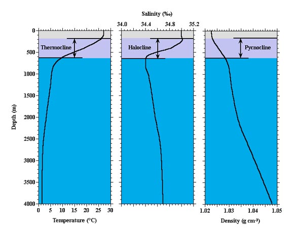 Some of you might be wondering about a bit aboutthe ‘stabilizing’ argument. I think this is basically explaining that ordinarily the top of the ocean is warmer than the lower depths and warmer water is so is less dense. If forcings heat the top layer making it even warmer that will tend to inhibit upwelling in places where cold water does upwell and down-mixing where that happens. )
 Watanabe continues:
It is not yet clear why the heat uptake efficiency is strengthened in nature. Although the enhancement of heat uptake could be induced by natural variability (Figure 3), consistent with better reproduction of hiatus with initialized hindcast experiments [Meehl and Teng, 2012; Guemas et al., 2013], it could also be the result of anthropogenic forcing. In the Southern Hemisphere, surface heat appears to penetrate at around 50 S (Figure S2), where the wind-induced Ekman down welling may have intensified in recent decades in associ-ation with stratospheric ozone depletion [Thompson and Solomon, 2002]. We cannot yet conclude whether the observed hiatus was part of unpredictable natural phenomena or a deterministic response to predictable changes in external forcing agents. However, the decrease of k represents a physically based response of the climate system to GHG increase, as inferred from the results in GCMs. Therefore, unless models miss effects of other forcing agents, it is likely that this process will occur and act to accelerate surface warming in coming decades
Above he now explains that ‘k’ increasing could either be due to ‘natural variation’ or it might merely be due to the argument about surface heating stabilizing being insufficient. But then he goes on to say that — based on climate models- we do expect ‘k’ will decline if forcings are positive. So unless the climate community is wrong about forcings being positive, we should expect ‘k’ to begin to decline. In which case, we should see accelerated warming in coming decades. (I infer the acceleration would be due both to the positive forcings and to ‘k’ finally declining as expected if forcing is positive.)
I think this ought to give some people a bit to chew on. Obvious questions are: What did cause the observed decrease in k to a level outside the range indicated by climate models. While discussion of the physical mechanisms is interesting, I’m not entirely sure this gets us much futher along in ‘explaining’ the hiatus. After all: we started with recognizing the recent observed trends are outside the range consistent with models. The three possible explanations for that are: (a) natural variability, (b) forcings are wrong or (c) models can’t reproduce the correct distribution of surface temperatures given correct forcings.
Watanabe then tries to explore (a). We finish by seeing that the magnitude of the ‘k’ parameter is high giving a somewhat plausible physical explanation. But then the ‘k’s move in the opposite direction predicted by models and are outside the range consistent with models. And the three possible explanations for that are: (a) natural variability, (b) forcings are wrong or (c) models can’t reproduce the correct distribution of ‘k’ given correct forcings.
1. Strengthening of ocean heat uptake efficiency associated with the recent climate hiatus Masahiro Watanabe,1 Youichi Kamae,2 Masakazu Yoshimori,1 Akira Oka,1 Makiko Sato,3,4 Masayoshi Ishii,5 Takashi Mochizuki,6 and Masahide Kimoto1 Received 30 March 2013; revised 5 May 2013; accepted 6 May 2013
Thank you Lucia.
You said: “This would tend to support the notion that the slowdown could be due to natural variability rather than other possible explanations like ‘the sun’, ‘volcanic aerosols from small eruptions’, ‘asian brown cloud’ or even ‘there is no warming’.”
I always lump things like the sun and volcanic aerosols into natural variability. In other words, if it is caused by humans (like the asian brown cloud) that is not natural variability – but everything which happens normally, which is not caused by humans, is part of natural variability.
You appear to be using a different definition of natural variability than I am -and I thought I would inquire – what is your definition of natural variability?
lucia,
But doesn’t that imply that the heat content of the top layer has to increase in order to get more down-mixing? Yet the ARGO data says the 0-700m layer heat content has been flat. I must be missing something.
RickA–
Yes. I mean “ENSO/PDO etc type natural variability”. That is: variability that arises in absense of any changes in external forces. I don’t know of vocabulary to distinguish between the two types of natural variability. Are you aware of a term? I’d be happy to adopt one but in the mean time, the same word seems to get used for both. (This is confusing. But that does happen with other words in English too.)
All other things (including salinity) being equal, if the top layer gets warmer you should have less down mixing (in terms of ‘k’ declining. The product “kδT” might still increase). The reason is:
1) If water at the top is less dense, the momentum of cool fresh upwelling water will slow as it hits the less dense regions and so this column will upwell less quickly. So, ‘k’ should decline.
2) When wind is driving mixing resulting in turbulent diffusion, the bouyancy will tend to make “warm” packets want to “rise up” thereby inhibiting mixing. So, ‘k’ should decline.
I think that’s the argument. Or course the total product “kδT” could increase. (No one is arguing the effect of the temperature gradient is sufficient to make that change sign. That would be beyond odd.)
DeWitt Payne (#116605)
“the ARGO data says the 0-700m layer heat content has been flat.”
Watanabe et al. write “upper-ocean heat content is shown to increase continuously after 2000.” So they don’t view upper OHC as flat. Its rate of increase may have lessened (assuming that one can usefully compare the pre-Argo data to current Argo data). But still positive, according to Levitus et al.
Lucia:
I am not familiar with a term for this.
I do find it confusing though.
A volcano changes the external forcing by not letting as much solar energy reach the ground. The same amount of energy is hitting the Earth – but more is being reflected (that is my understanding).
Doesn’t ENSO/PDO also affect clouds (and/or the jet stream), and therefore also change the external forcing (in the sense you are using that term)?
Isn’t the 11 year sun spot cycle a change in external forcing? But you consider that natural variability to be different in kind from ENSO/PDO type natural variability?
I guess I was not aware that anybody subdivided natural variability into different types – so this caught me off guard.
To me, ice ages (malkanvich cycles), eruptions, ENSO/PDO, lightning caused fires, solar variations, are all natural, in the sense that human caused climate change is unnatural (i.e. wouldn’t happen if we were not here).
Killing all the bison (less methane), carbon black (changes albedo), human emitted CO2 and methane (more cows, for example)(GHG’s), cities, deforestation, air conditioning, CFC’s, smog – etc. are all things which are caused by humans being here and therefore “unnatural” and not part of natural variation.
So perhaps I have not been nuanced enough (for years apparently).
Anyway – I thought this point was interesting.
RickA (Comment #116616)
Maybe. But that’s qualitatively different from the sun itself putting out less heat or the volcanoes acting like an “umbrella” and the placement of that umbrella being entirely independent on the current state of the “weather”.
Any ENSO/PDO cloud thing is specifically a linkage of world-wide weather patterns of different types (e.g. Temperature, humidity, precipitation, evaporation) exciting themselves. In contrast, the volcano blows when it blows.
Agreed. Those are all unnatural in the strictest sense. But there is still a distinction between “solar/volcano” and “ENSO/PDO” variability.
Re: HaroldW (Jun 20 10:16),
Flat was a bit of hyperbole. But the ARGO data has the 700-2000m heat content rising almost twice as fast as the 0-700m heat content. It also led to a step change in the calibration curve for 0-700m steric sea level vs heat content that is, AFAIK, still unexplained. Something smells wrong.
Lucia, I like to differentiate between Internal Natural Variability (ENSO,PDO,AMO) and “external” or Forcing Natural Variability (Volcano,Sun,Clouds) on changes levels of forcing one changes distribution of heat. Both are natural.
Second I never see any of these studies mention that an increase in heat uptake in the Tropics (at least for most of the year)would just increase evaporation and would actually add nothing to Ocean heat content. Heat them faster and the afternoon thunderstorm just comes 5 minutes earlier. any “gain” in uptake would need to be extra-tropical. I wish they would have broken the analysis down in latitudinal bands.
I don’t understand the empirical aspect of the paper if any. Is it merely a claim that because the models missed the hiatus, and we assume that the predicted heat increase has to still be in the sytem somewhere and since it is not in the air or sea surface layers, it must have been rapidly deposited in the deep ocean without appreciably warming the top layers and effected in a manner unanticipated by any of the models?
Given that we don’t have any detailed measurements of deep ocean temps and that total atmospheric heat content is magnitudes less than a rounding error of ocean heat content, it seems that speculation about the role ocean heat content is almost as pointless and as irrefutable as the model ensemble itself.
Lucia – “unforced” and “internal” both seem to describe the type of variability we are looking at. you can pick at these, but they seem to be the standard terms and fit well enough with the qualitative difference you mentioned..
Any reason I can’t use the arrow keys on my keyboard any more inside of the comment box?
SATg  î€ î€‚ . ???
Nu language?
Or just my browser?
(not rhetorical, just confused)
If and when climate models are ever capable of simulating coupled ocean-atmosphere processes, such as ENSO, then studies such as Watanabe et al (2013) will have merit. Until that time, they do not. They’re simply computer-aided speculation.
I would suggest that above interpretation could be erroneous. Ocean temperature oscillations in the North Atlantic (AMO) trail Arctic Atmospheric Pressure change by approximately 6-8 years.
http://www.vukcevic.talktalk.net/AMO-NAO.htm
the above may be associated with the Arctic ice formations drifts.
It takes ice about 6-10 years (min 6 years) to drift from the Beaufort Sea to the Fram Strait. Sea ice from the Kara Sea region reaches Fram Strait in 2 to 4 years (min 2 years) while sea ice from the Laptev Sea takes roughly 3 to 6 years (min 3 years) to reach Fram Strait.
Fram Strait is the embryonic AMO index area.
“The Strait represents the unique deep water connection between the Arctic Ocean and the rest of the world oceans. Its bathymetry controls the exchange of water masses between the arctic basin and the North Atlantic. The significant heat flux through water mass exchange and sea ice transport, i.e. transport of fresh water and sea ice southwards and transport of warm saline waters northwards, influences the thermohaline circulation at a global scale.” Alfred Wegener Institute
Ben
Clouds are internal variability.
George
The empirical aspects are:
1) The compared the observed 10 year trend to those in models and found them outside the range for models. Observed trends are empirical.
2) They estimated the ‘k’ that would apply to a fit using observations and using models and compared the two. The ‘k’ based on observations is empirical (or at least semi empirical.)
There is also a sentence I didn’t quote that looks at radiative balance in models vs. observations:
So the conclude that heat must be accumulating somewhere.
Imperfect cut and pasting form the pdf at GRL.
Lucia,
Interesting post.
.
“But then the ‘k’s move in the opposite direction predicted by models and are outside the range consistent with models. And the three possible explanations for that are: (a) natural variability, (b) forcings are wrong or (c) models can’t reproduce the correct distribution of ‘k’ given correct forcings. ”
.
Ummm.. I am betting the climate science community will either ignore the paper or support option (a), just like F&R do. Wait, F&R’s sources of natural variability have nothing to do with ocean heat uptake!
.
I find it more than a little amusing so many excuses for the recent temperature divergence can be generated, while the simplest one (the models are way wrong, so their temperature projections are mostly useless) seems to be never seriously considered.
Lucia,
Another humorous observation: “That this is a statistically rare event in models is the exact opposite impression from the one given by Trenberth and discussed here and here. ”
.
Which nicely parallels that both exceptional heat and exceptional cold are due to global warming; just like the lady from the COOK Islands said! (http://rankexploits.com/musings/2013/summer-is-cold-proves-global-warming/)
Re: lucia (Jun 20 11:29),
Clouds as a reflector of incoming radiation would not be internal variability if the amount and location of clouds are driven by external factors i.e. cosmic rays.
Other cloud variations are symptoms of ENSO PDO ect.
Tomato tomaato
Ben
Internal variability is not defined by whether something affects the amount of incoming radiation that hits the earth. It is defined by whether the feature is internal to the climate system.
Unless you think something external to the climate system is creating the clouds, they amount level and character of clouds is internal variability. In contrast, the current state of the earth’s climate does not affect the heat out put by the sun and it does not cause or inhibit volcano eruptions.
BTW: The model used to do the linear regression on SST vs SATg is Miroc 5. This was not in the AR4 ensemble (which is fine). But it’s interesting to note the sensitivities.
Miroc5 has a somewhat loser sensitivity that Miroc3.2.
http://journals.ametsoc.org/doi/full/10.1175/2010JCLI3679.1
“So they conclude the heat must be accumulating somewhere.” Just like Trenberth. Based on a statistical model -in Bob Tisdale’s words ” computer aided speculation”- and under 700m without any ARGO [best spatial distribution of any ocean data gathering system we have] trace of the gazilliojoules on their way down between 0 and 700m.
I’m with Dewitt Payne on this one: doesn’t look right and doesn’t smell right. Like being sold flounder for halibut.
“Ben (Comment #116619)
June 20th, 2013 at 10:43 am
Lucia, I like to differentiate between Internal Natural Variability (ENSO,PDO,AMO) and “external†or Forcing Natural Variability (Volcano,Sun,Clouds) on changes levels of forcing one changes distribution of heat. Both are natural.
Second I never see any of these studies mention that an increase in heat uptake in the Tropics (at least for most of the year)would just increase evaporation and would actually add nothing to Ocean heat content. Heat them faster and the afternoon thunderstorm just comes 5 minutes earlier. any “gain†in uptake would need to be extra-tropical. I wish they would have broken the analysis down in latitudinal bands.”
################
The data is available. dont give homework to other people.
If you are incapable of doing the work, dont comment.
Mosher,
I think that applies to giving homework to other people on the blog. Wishing “they” would have done it (as in the authors of a paper) is pretty legit I think. I would 1) support the comment 2) I’m capable of doing the work 3) have no inclination to do so.
Still wondering why I can’t use the arrow keys. Actually that’s not the issue, it’s that I can’t move the cursor indicator with either the arrow keys or the mouse. I can move the active typing position using either but the visible cursor stays put.
lucia, I get Miroc5’s sensitivity may be less constrained, but I don’t think that makes it a loser 😛
BillC, when I say, “I wish I had a million dollars,” don’t you know I’m actually telling you to give me a million dollars?
BillC/Ben,
I think it’s likely the authors of this didn’t do whatever analysis Ben wants them to do with latitudinal bands because it’s not relevant to their investigation. (Or at least I don’t see how it’s relevant, and I don’t know why they should have thought it relevant.)
Miroc 5 seems to have lower sensitivity. I was thinking more along the lines of this might explain the existance of “flat bits”. Tomorrow I’m going to download a bunch of CMP5 data. Does anyone have an R script to make it easy. (It’s not that hard manually… but if anyone has it… : )
You only clearly see the ENSO influence on global OHC if you divide the world ocean into two subsets, the one following the swings of the western (Warm Pool) sector vs. the one following the swings of the eastern (NINO3.4) sector – the ‘Extended Indian-Pacific Warm Pool’ (covering slightly more than one fifth of the total area of the ocean) and the ‘Rest of the World’ (slightly less than four fifths) respectively; map:
http://i1172.photobucket.com/albums/r565/Keyell/world-map-2_zpsd5298cf2.png
Red area is the West Pacific/East Indian Warm Pool, extended west and southwest + the SPCZ extension in the South Pacific and the KOE in the North Pacific.
This is the OHC (0-700m, NODC) evolution during the ARGO era in the two subsets juxtaposed (note, the blue ‘Rest-of-the-World’ curve to the right is scaled up to accommodate for the much larger area covered):
http://i1172.photobucket.com/albums/r565/Keyell/OHCglhotcold_zpscd8c7d78.png
Something steplike happens in 2008 in both regions, a shift of some kind going the opposite way. But besides that, watch how both curves correlate to the NINO3.4, albeit the red Warm Pool one in an inverted fashion.
BTW, the apparent shift in 2008 seems to correlate well with a general shift in the pressure gradient west-east in the Pacific (SOI):
http://i1172.photobucket.com/albums/r565/Keyell/SOI_zps4a244c80.png
Watch how the pressure differential fell across the 1976/77 Pacific Climate Shift.
A less steep pressure gradient from west to east would lead to on average weaker zonal wind stress across the ocean surface and hence less mean evaporation (latent heat loss), though mainly in the central/eastern part (the NINO3.4 sector), not necessarily in the western (Warm Pool sector).
A steeper pressure gradient, which we saw returning around 2008, would enhance the advection from the eastern to the western Pacific, relatively cooling the former and warming the latter.
What is the difference between this paper’s analysis and post hoc rationalization?
DeWitt Payne said
“But doesn’t that imply that the heat content of the top layer has to increase in order to get more down-mixing? Yet the ARGO data says the 0-700m layer heat content has been flat. I must be missing something.”
No, there is another possible mechanism. Increased heat flow downward can occur through a combination of two factors. Because the volume of water moving is unchanged but it has a higher heat content per M^3, or because its heat content is unchanged but a larger volume of water is being moved.
In the latter case this wouldn’t show up in the ARGO data for the surface.
And this is what is believed to be happening. The major ocean gyres, one in each ocean basin, psh water towards their centers where it then downwells through a process called Ekman Pumping. And the gyres are created by the winds. Particularly the Trade winds near the Equator blowing from the East and the Roaring Forties blowing from the West.
It is being suggested that the increase in downwelling of heat is correlated with an increase in the Trade winds which could then spin up the gyres and increase the downwelling. And the climate models aren’t doing that well at predicting the increase in the Trade Winds so they don’t predict the increased downwelling that well.
But as sequestration of heat to greater depth continues, the increasing buoyancy at depth as a result would provide a counter balancing force to the Ekman pumping and eventually slow it down again.
It is quite possible that there is a natural oscillation in this pattern of Trade winds/gyres/downwelling and that we see this manifested in things like the PDO.
Nothing much. But science actually involves a sizeable amount of post hoc rationalizations. The post hoc rationalizations that later turn out the be predictive are kept. The others get cast aside. That said: We won’t know for sure whether the event is a bump before a dramatic increase or evidence of lower sensitivity until later on. Unlike other fields we can’t do a physical experiment in the lab to find out.
Lurker writes “What is the difference between this paper’s analysis and post hoc rationalization?”
Maybe someone should rationalise actual falling temperatures now so that if they happen it will be in line with theory and nobody will be able to criticise them for “post hoc rationalizations”
.
But why stop there. May as well do sea level rise and precipitation, changes to PDO and so on.
It could be the “I have my cake and I’m going to eat it too” paper.
Re: Glenn Tamblyn (Jun 20 20:00),
Higher heat content means higher temperature. The patterns you describe should be discernible in the ARGO data. It should also show up in the depth of the thermocline, which is a bit easier to measure. Ekman pumping rate still depends on the temperature gradient. If you increase Ekman pumping and increase the upwelling flow, the gradient of the thermocline should steepen. If you increase Ekman pumping at a constant upwelling rate, the thermocline moves deeper. All these things should be obvious.
But that doesn’t explain apparent step change in the thermal expansion coefficient around 1996. IMO, there was no step change. In fact, they still haven’t properly reconciled pre-ARGO data with ARGO data.
DeWitt
Higher heat content means higher temps somewhere. But it doesn’t have to translate to higher temps at the surface. If heat is being removed from the surface as fast as it is being added at the top, no temperature rise occurs at the top. But temperature rise occurs at depth because more warmer water is being added there. ARGO can only detect temperature but not flow rate so it can’t tell us what the heat flow rate in/out of a particular volume of water actually is. We can only infer that from the temperature change in that volume.
If I have a water tank with a heater in it and I am pumping hot water out of that tank at a constant flow rate and replacing it with cold water my heater needs to be at a certain heat output to maintain the temperature in the tank. If I increase the heat output from the heater by 10% then the temperature of the water in the tank will rise. However, if I also increase the flow rate of the pump by 10% then the temperature in the tank doesn’t change, even though the total amount of heat being removed has gone up 10%. And I can’t detect this just from measuring the temperature.
And at the basic level, the patterns I describe are being discerned in the ARGO data – less warming at the surface, more warming at depth.
As for any thermocline changes, I don’t know whether that is expected or not. However I would expect that any changes would be confined to the upwelling and downwelling regions. If one were looking at the average thermocline depth over large enough areas this might well cancel out.
And the point about Ekman pumping rate was exactly my point about possible oscillations. If a changed thermal gradient tends to put a brake on the Ekman pumping, that might then force back to actually being a brake on the basic circulation of the gyres – if they can’t move water to the center, they can’t spin as fast.
One possibility is an oscillating phenomenon where they can spin up, more heat gets pumped downwards, the changed thermal gradient slows them again and the cycle repeats.
There is a massive amount of kinetic energy in the gyres so any such oscillation would not happen quickly – years to spin up and spin down again. This strikes me as at least a plausible explanation for the PDO and other cycles.
But if an outside force such as changes in the wind patterns is linked to this then you definitely have a mechanism that might produce an oscillation.
Any reality would be more complex than this but there certainly seems to be a basic mechanism there.
Here are some papers a friend pointed out to me that all have contributions to make in understanding these processes.
http://www.geo.arizona.edu/BGDL/articles/Russell_etal_2006b.pdf
http://www.image.ucar.edu/idag/Papers/Saenko_wind-driven.pdf
http://www.geo.arizona.edu/BGDL/articles/Toggweiler_Russell_2008.pdf
http://www.ncbi.nlm.nih.gov/pmc/articles/PMC3586712/
The first one, Russell 2006 is really interesting – two competing mechanisms that can speed up or slow down the process. Variations in those mechanisms have a lot of potential to create oscillations.
The science of this is all being developed but it has the potential to provide a much better explanation for a lot of climate variability. And collectively they suggest that the trajectory of surface warming won’t necessarily be steady, more likely step like, possibly even including periods of some surface cooling.
That’s why surface temp’s aren’t a very good metric for monitoring climate change. Whole of ocean heat content is the best. Currently we can go down to 2000 meters and I believe they are developing a really deep diving version of ARGO that can sample the rest of the ocean depths – can’t come soon enough.
@Lucia (and others)
With regards to “warm water” in the surface “blocking” upwelling.
With the caveat that others might have addressed the issue allready: I would think one of the major mechanisms for upwelling are (rather) persistent wind patterns “blowing” the surface water “away” (these wind-patterns are often directed off-shore”. The deeper water then simply compensates for the “missing water on top. If the wind-generated current (and water movement) is strong, I expect that such a system can “handle” quite large density-differences (be it from salinity or temperatures).
Cassanders
In Cod we trust
So we now know (again?) that the measured figures lie within those that the models could reasonably be expected to generate and still be correct.
Therefore the models ARE correct and the warming will resume.
lucia (Comment #116688)
June 20th, 2013 at 8:29 pm
lurker passing through, laughing (Comment #116683)
June 20th, 2013 at 7:11 pm Edit This Edit Delete
What is the difference between this paper’s analysis and post hoc rationalization?
Nothing much. But science actually involves a sizeable amount of post hoc rationalizations. The post hoc rationalizations that later turn out the be predictive are kept. The others get cast aside. That said: We won’t know for sure whether the event is a bump before a dramatic increase or evidence of lower sensitivity until later on. Unlike other fields we can’t do a physical experiment in the lab to find out.
Thanks. However it seems those devoted to promoting the idea of “AGW = global climate catastrophe” have crossed the border between post hoc rationalization and making excuses.
lucia (Comment #116660)
June 20th, 2013 at 2:07 pm
“Does anyone have an R script to make it easy. (It’s not that hard manually… but if anyone has it… : )”
Lucia, it has been a while since I did this but here is a script I found. As I recall, the RCP scenario runs are all located together in the link, like I show for rcp60, below. Once you get that link for downloading you can do your own thing with the data.
Url=”http://climexp.knmi.nl/data/icmip5_tas_Amon_ens_rcp60_0-360E_-90-90N_n_su_+++a.txt”
download.file(Url, “CMT”)
RL=readLines(“CMT”)
Mrg2=round(seq(from=1850, to=2300-1/12, by=1/12),digits=3)
for(i in 1:47){
Exp1=expression(i-1)
if(i10 & i100) {Idx1=paste(“# ensemble member “,eval(Exp1))}
Exp2=expression(i)
if(i9 & i99){Idx2=paste(“# ensemble member “,eval(Exp2))}
Mat1=match(Idx1, RL)+2
if(i==47){Mat2=length(RL)-1} else{Mat2=match(Idx2, RL)-2}
Series=RL[Mat1:Mat2]
writeLines(Series,”Temp.dat”)
Ser1=round(read.table(“Temp.dat”),digits=3)
Mrg2=merge(Mrg2,Ser1, by.x=1, by.y=1, all.x=TRUE)
}
CName=read.table(“clipboard”)
CN=as.character(CName[,1])
colnames(Mrg2)=c(“Time”,CN)
write.csv(Mrg2,file=”RCP60_CMIP5_All_47_Model_Runs_Includes_Multiple”)
#The clipboard was to a table I generated in Excel to relate model names to codes that allowed replicate model runs to be identified.
Is the TOA energy budget showing a continuous 2 decade excess and used to conjecture about heat transport to ocean depths well observed and modeled from a quantitative perspective? I recall seeing a recent post at one these blogs by TroyCA where the implication was that the TOA energy budget was not well quantified and that the “missing” heat in the oceans per the climate models was predicated on what climate models predict for the TOA energy budget.
“What is the difference between this paper’s analysis and post hoc rationalization?”
While papers do this to a degree, I get the idea that this paper does a lot of hand waving only to – in the end – conjecture that yes indeed the warming hiatus can be affected by a change in ocean heat uptake efficiency and that the models over the long run have physical reasons for that efficiency to decrease. It avoids talking about the implications of sensitivity.
@Glenn Tamblyn
Regarding the Ekman suction/pumping, is it acceptable to think of this as the ocean’s Hadley Cell. That is, a corkscrewing of the sea running east to west, with the top of the “cell” reaching just below the surface in the tropics and the poleward edge reaching out to ~40 degrees. One cell in each hemisphere.
A couple of years ago I was looking at the ARGO gridded data and generated an image plot showing relative temperatures by latitude and depth which seemed to indicate this:
https://sites.google.com/site/climateadj/argo-sine-fitting/sine-mean-argo.png
Cassanders (Comment #116704)
June 21st, 2013 at 1:14 am
“If the wind-generated current (and water movement) is strong, I expect that such a system can “handle†quite large density-differences (be it from salinity or temperatures).”
As it happens, I’ve just started (two days ago) to look at the relationship between NINO3.4 and salinity using 8 years of ARGO data. Not much to report so far except it looks like surface salinity lags temperature by a month or two. These are highly correlated within the NINO3.4 zone, but with an even higher anti-correlation just to the west. The correlations to the east are lower. Maybe I can find eastern salinity leading NINO3.4, but I suspect that the temperature itself would be the better predictor. I haven’t looked at the potential density data yet. So for now, I also think that the wind is the primary driver of this particular oscillation. Of course, everything is coupled.
AJ
I lobster and never flounder
AJ,
I think if the amount of hand waving by AGW apologists was converted to atmospheric activity, we would get a pretty good breeze.
Glenn Tamblyn
Unless I’m missing something in your reply to DeWitt, you appear to be arguing that it is actually possible for joules/calories/heat [call it what you will] to make their way down through the upper 700 meters of all the oceans around the world [70% of it’s surface not to mention the volume involved] without this showing up in the ARGO data -which, it bears repeating, is the absolute best three dimensional spacially distributed oceanic data we have.
I think that it is stretching credulity just a tad too much to ask people simply to accept that this process does not show up in the data gathered by over 3000 state-of-the-art sensors.
“Transmutation” comes to mind and until Trenberth, you or others can come up with a verifiable, repeatable experiment that demonstrates how this heat transfer actually occurs without leaving a trace on the way down, as far as I’m concerned [and a good number of others I’ve discussed this with] Trenberth’s “hiding heat” has the makings of alchemy, homeopathy, astrology, desperation or fish gut reading. Your pick.
Re: Glenn Tamblyn (Jun 20 22:10),
Your tank example is flawed. The ocean is a closed system. The hot water drained from the tank has to go somewhere in the same system and the cold water has to come from somewhere in the same system. In the simplest case you need a supply tank with a refrigerator. So then things become more complicated. What’s the temperature of your cold water and how much heat has to be removed to maintain that temperature because the hot water you remove from the heated tank is pumped back into the refrigerated tank.
But I do agree that ocean heat content is the best measure we have of radiative imbalance. I’m just not convinced that the measurement system has all the bugs worked out of it yet. See for example MSU temperature retrieval by satellite and orbital drift. Do we know that the ARGO floats are randomly sampling the ocean volume or do currents tend to concentrate them in areas with particular conditions like downwelling areas.
Is there a lab experiment that could be done physically showing how radiant heat moderated through atmosphere can heat water at depth?
lurker–
I’m sure the people interested in solar energy have done it. Others have done things too. Why?
In point 3 Lucia suggests
“he is suggesting that in models these periods are associated with enhanced ocean heat uptake relative to the normal rate.”
except what I read in the quote is if they force increased ohc to mimic the obs then they get increased ohc uptake. Just about as circular an argument as you can get.
So if they are suggesting a subset of the GCM models might be barely capturing the hiatus with their internal variability then why not take this subset and use it to investigate the earlier warming period to see what sort of insight it might give us to the role of internal variability in that warming phase as well?
Can’t help thinking they just want to explain away a problem rather than shed light on the climate record as a whole.
(BTW the first line made me laugh a little (lal??). Teh use of “apparently slowed” suggests some doubt about the various temperature records to give us a true measure. The sort of wording you might see on WUWT or similar)
DeWitt
My tank example is only intended to illustrate that one can get increased heat transfer through fluids without requiring an increased temperature at the origin.
Are the ARGO floats random. Obviously not fully so. However, athey only need to be sufficiently random to give adequate coverage since area weighted averaging would be a standard part of any processing algorithm.
And the floats aren’t just left. Oceanographic research vessels from the nations in the research consortium are routinely picking up damaged floats, releasing new ones etc. Maintaining an adequate spread would be a standard part of such a process. Obviously if left for too long they would all start to concentrate in the center of the gyres, along with all the floating plastic.
Here is there current distribution, updated daily
http://w3.jcommops.org/website/Argo/viewer.htm
Looks pretty well spread to me.
Wantabe serious ?
the recent observed trends are outside the range consistent with models. The three possible explanations for that are: (a) natural variability, (b) forcings are wrong or (c) models can’t reproduce the correct distribution of surface temperatures given correct forcings. or how about
[d] Lucia ” other possible explanations like ‘the sun’, ‘volcanic aerosols from small eruptions’, ‘asian brown cloud’ or even ‘there is no warming’.”
What Wantabe is trying to say is that the models are correct and that the observations are systematically biased to produce a warmer surface for a particular reason. The observations will come to realise that they are wrong in time and will then approach the mean of the correct model ensembles as they release the heat they have hidden in the sea by the magical conveyor belts of Namor [ meridional overturning circulation ]
Due to the multitude of factors no model can correctly predict the future for 1, 100 or a 1000 years . But the climate is repetitive around a random walk and a guesstimate can be made 1-10 yearly with excellent hopes of modest approximation. All such models should be primable with yearly input changes to reflect the actual climate changes and improve the ongoing results from that new point in time.
All models [Mosher] should predict at worst 4 out of 10 years of falling temps in a year, practically 4.999 out of 10 If we are in an increasing warmth epoch. If the solar minimum reduced solar input occurs as predicted and temps are more likely to go down on average models should still predict nearly 5 warming years to 5.001 cooling years.
All models are wrong is a good fun line but when all models are uniformly wrong then there is an inbuilt warming error [or conclusion]. We know what this is. It is accepting a 0.2 warming per decade CO2 induced with multiplications.
You can work it out by taking the average trend of the spaghetti graph average [Tamino and Lucia and Mosher].
The mean ensemble average is good as it shows the inbuilt bias of all current models. GIGO is really WIWO.
The research results of Watanabe at al claim that the ocean has been adjusting its heat uptake in the last few years as a result of transient changes in the large-scale hydrodynamics. This has the effect of suppressing the warming in terms of temperature, although the heat uptake from the AGW forcing still exists. So the implication is that what is lacking in a temperature rise is made up for by the heat sinking of the ocean.
The ocean heat uptake efficiency measure of Watanabe is related to the ratio f between ocean and land temperature defined on my blog post
http://theoilconundrum.blogspot.com/2013/05/proportional-landsea-global-warming.html
The idea is that — similar to the aim of the Japanese research study — to see if we can detect changes in f over the last few years.
To do this we need to take great care with the numbers. Instead of using the WoofForTrees data, I used the CRU data directly. The sets were CRUTEM4 (Tl=land), HadCRUT4 (TG=global), and HadSST3 (To=ocean). The composed set looks like the following chart for a value of f = 0.5, which is the nominal fraction assumed for the original proportional land/sea analysis.
http://img534.imageshack.us/img534/1622/5vj.gif
The composed temperature lies on top of the HadCRUT4 global temperature
If we look at the error residual between the HadCRUT4 global temperature and the fractionally composed model, we get the following chart. Note that as an absolute error, the value is obviously decreasing over time, likely attributed to better and more accurate record keeping with current temperature measurement techniques.
http://img189.imageshack.us/img189/5863/uvt.gif
The absolute error decreases with more recent records.
(The last data point is 2012, which often undergoes corrections for the next update.)
The high resolution and low error in recent years indicates that perhaps we can try to more accurately fit the fraction f. So essentially, we want to zero out the error by solving the proportional land/sea warming model for a continuously varying value of f.
0=TG-1/2(f*po+pl )Tl+ 1/2(po+pl*f)To
This turns into a quadratic equation for f, which we can solve by the quadratic formula. The set of value calculated by minimizing the error is shown below. Note that the average remains around f = 0.5, but it shows a distinct decreasing trend in recent years.
http://img442.imageshack.us/img442/4509/n5t.gif
The fraction ratio of ocean to land temperature appears to be decreasing in recent years, leading to an apparent flattening in global temperature rise. Lower values of f cause the global temperature signal to appear cooler for a given AGW forcing.
If this is a real trend (as opposed to some type of accumulating systemic error or noise) it is telling us that more of the heat is accumulating in the ocean, consistent with the claims of Watanabe et al. It is possible that the fraction is actually decreasing from a past value of around 0.6 to a current value of 0.4. Although this is a subtle effect in terms of the fit (probably the not most robust metric one can imagine), it has significant effect in terms of the global surface temperature signal.
This is seen if we deconstruct the proportional model in terms of the land temperature alone, assuming the area land/ocean split as po/pl=0.71/0.29 :
TG = (0.71*f+0.29)Tl
Note that with a slowly increasing land temperature signal Tl , the declining f can compensate for this value and actually cause the global temperature value TG to flatten.
To take an example, reducing the value of f from 0.6 to 0.4 causes the global temperature to decline from 0.716*Tl to 0.574*Tl. If the land temperature is held constant, the global temperature will decline, while if the land temperature rises by 25%, the global temperature rise will look flat.
That is exactly what Watanabe et al are claiming. Moreover, they assert that this decline can’t remain in place for the long term, and eventually the ocean hydrodynamics will stabilize or even reverse, with a concomitant rebound in global temperature.
To review, the essential premise of the proportional land/ocean model is:
1. The land surface reaches the steady-state temperature quickly
2. The ocean sinks excess heat, thus moderating the sea surface temperature rise.
3. The fractional ratio of ocean temperature to land temperature is given by f.
4. The global surface temperature is determined as combination of land and sea surface temperatures prorated according to the land/sea areal split.
From this set of premises, we can algebraically estimate the amount of ocean heat sinking from global temperature records as gleaned from the Climatic Research Unit.
Re: WebHubTelescope (Jun 22 11:53),
My problem with that hypothesis is that increased rate of energy accumulation in the ocean should have been reflected in the sea level rise, particularly the big jump in OHC between 2000 and 2004. It doesn’t appear to be. That would mean, if the hypothesis were correct, that sea level rise due to ice melt and pumping from slow refilling aquifers was reduced by exactly the same amount that steric sea level rise increased. That seems unlikely to me.
Re: Glenn Tamblyn (Jun 22 03:45),
Sure. But in the real world, a change in flow has other consequences which are, at least in principle, observable. They are things like the average depth and temperature profile of the thermocline. When I see publications that show that these changes are occurring, I will be more prone to accept the hypothesis that the ‘missing’ heat is going in to the deeper ocean rather than it doesn’t exist at all because of, say, a slight increase in albedo.
WebHubTelescope (Comment #116836)
June 22nd, 2013 at 11:53 am
If I do a regression from 1998-2011 on f from your graph I obtain an R^2=0.037 and a p.value (for a slope different than 0) =0.49.
Watanabe’s paper discussed here appears to be very intent on showing that:
1. Most important is that the efficiency of heat uptake by the oceans can be shown physically and from the models to be decreasing generally with increases in GHGs in the atmosphere, i.e. the warming trend will have to continue at some future time with increased GHG emissions.
2. The current pause in warming is probably an internal phenomena related to a change in the efficiency of heat uptake by the oceans. The operation of this phenomena is currently not understood by the models (modelers) or others. If it is related to anthropogenic causes it would necessarily be a “new” phenomena.
Further the paper is rather vague in my judgment about some aspects of the problem in the following areas:
1. The paper talks about climate models and the variations in trends over 10 year periods and appears to relate the greater variation in trends within model replications as a better capability of the model to capture natural variations in temperature. If the change in heat efficiency is a new phenomena presumably not taken into account by the models then I do not see a connection between decadal trend variations and the current hiatus in warming. I would have hoped that the Watanabe paper would have been more clear on this point.
2. The paper uses the TOA estimates and the efficiency of ocean heat uptake and plays with them without a big shout out to the uncertainties involved and any consideration to how sensitivity might enter into the puzzle.
Below is the TroyCA comment for which I was looking. It was on the thread here at the BB titled: “The “D†word: Alternative definitions”. The comment was in reply to a comment from Neal J. King which I also included:
Troy_CA (Comment #115521)
June 10th, 2013 at 11:47 pm
Neal J. King comment:
“The point is that if you calculate how much sunlight is arriving, subtract off the reflection (albedo factor), and subtract off the power radiated out (satellite measurements), what’s left must have been absorbed somewhere. When the surface temperatures are not rising fast enough to justify this, you can look in the oceans; and they have the Argo system that takes temperature measurements down to 2000 meters. They can measure the temperature as a function of depth and find that 70% of what was missing above is in the layers 0 to 2000 meters; and there is good reason to believe that the remaining 30% is going below 2000 meters, where you can’t see it.”
TroyCA reply:
“Chiming in one more time, I think it is important to note we are NOT simply able to say that “what’s left must have been absorbed somewhere†because we don’t know “what’s leftâ€. The satellite estimates of albedo and “power radiated out†are definitely not accurate enough in absolute terms, which is the reason that the rate of ocean heat uptake is used to measure the TOA radiative imbalance, NOT satellites. In fact, in the primary satellite system, CERES EBAF, the “the global net [TOA imbalance] is constrained to the ocean heat storage termâ€. In other words, the absolute energy imbalance for that system is calibrated against the rate of ocean heat uptake…it is only in the interannual variations that the satellites provide a potentially higher degree of accuracy (see Loeb et al., 2012 for more discussion), but they give very little insight on the actual “power radiated out†for the purposes you mention.
Obviously, if the satellite measurements were able to diagnosis the absolute TOA imbalance and we noted that it was 30% higher than what we observed based on ocean heat uptake in the top 2000m, it would be reasonable to conclude it was absorbed somewhere below. Unfortunately, what is referred to as “missing heat†often comes from the expectation that the TOA imbalance should be higher if the earth is really as sensitive as the models suggest (and it should be), but rather than entertaining the possibility that the GCMs may generally be too sensitive, it is posited that the TOA imbalance really must be higher than observed in the top 2000m and the heat being absorbed elsewhere. Of course, that does little to change the GCMs that DO show a much larger amount of ocean heat uptake in the top 700m than observed, which leaves the speculation of “missing heat†not only shaky on observational grounds but theoretical grounds as well. It’s not impossible, but I certainly wouldn’t consider it likely.”
DeWitt said:
Good point. What is the estimated additional rise for a given increase of thermal energy?
I get this expression for steric sea level rise
SLR = alpha * dE / cp
where alpha is the volume coefficient of thermal expansion for water, dE is the excess thermal energy entering the ocean per area, and cp is the heat capacity of water per volume. Assume all of the volume expansion goes into a linear increase due to the container constraints.
Over the course of 10 years with an average excess of 0.1 W/m^2, I get around 2 mm of extra rise.
Over this same period, the sea level has risen 40 mm
http://sealevel.colorado.edu/
I may not be doing this correctly so corrections welcome.
I did parenthetically say that the graph of f is “(probably the not most robust metric one can imagine)”, but we don’t have a lot else to go on. It is essentially straightforward algebra and I could probably get analytical error margins by doing an uncertainty propagation on the quadratic formula solution. I also implied that the narrowing of the variance is “attributed to better and more accurate record keeping with current temperature measurement techniques”. That’s what this figure was about showing:
http://img189.imageshack.us/img189/5863/uvt.gif
The R^2 technique is likely not valid for non-stationary series such as this. Perhaps what I should do is a calculation in variance of f over time intervals, and then show how this is decreasing.
The comparison of land temperature and SST is appearing to gain importance in understanding global warming trends, and I hope that this helps with the understanding at the mere-mortal level of knowledge.
Webster, “Perhaps what I should do is a calculation in variance of f over time intervals, and then show how this is decreasing.”
Then there will be the Antarctic interpolation problem which adds variance after 1955. You will have at least 0.125 uncertainty trying to pick out a 0.0125 or less signal.
“The R^2 technique is likely not valid for non-stationary series such as this. Perhaps what I should do is a calculation in variance of f over time intervals, and then show how this is decreasing.”
Series with deterministic trends are never stationary – trend stationary yes – yet we calculate R^2 for trends and p.values which in this case implies that the probability of the seeing this trend when the trend is actually 0 is a 50-50 proposition.
But if you care to put some CI limits on your graph, I would be interested in seeing that done.
tetris (Comment #116745)
June 21st, 2013 at 11:17 am
Glenn Tamblyn
Unless I’m missing something in your reply to DeWitt, you appear to be arguing that it is actually possible for joules/calories/heat [call it what you will] to make their way down through the upper 700 meters of all the oceans around the world [70% of it’s surface not to mention the volume involved] without this showing up in the ARGO data -which, it bears repeating, is the absolute best three dimensional spacially distributed oceanic data we have.
I think that it is stretching credulity just a tad too much to ask people simply to accept that this process does not show up in the data gathered by over 3000 state-of-the-art sensors.
“Transmutation†comes to mind and until Trenberth, you or others can come up with a verifiable, repeatable experiment that demonstrates how this heat transfer actually occurs without leaving a trace on the way down, as far as I’m concerned [and a good number of others I’ve discussed this with] Trenberth’s “hiding heat†has the makings of alchemy, homeopathy, astrology, desperation or fish gut reading. Your pick.
lurker, passing through laughing (Comment #116776)
June 21st, 2013 at 2:55 pm
Is there a lab experiment that could be done physically showing how radiant heat moderated through atmosphere can heat water at depth?
lucia (Comment #116777)
June 21st, 2013 at 3:03 pm
lurker–
I’m sure the people interested in solar energy have done it. Others have done things too. Why?
Lucia, the modellers aren’t interested in solar energy – they have excised the direct heat from the Sun and claim that shortwave heats matter of land and oceans.
They claim the Sun is 600°C, from some weird planckian manipulation where they have taken the 300 mile wide band of thin visible light around the Sun to calculate its temperature – the Sun is millions of degrees centigrade.
They give two reasons why the direct heat which is longwave infrared from the millions of degree hot Sun doesn’t reach us, that the Sun isn’t millions of degrees hot, but only 6000°C so gives off insignificant radiant heat, longwave infrared and we get insignificant of insignificant, and/or,that the direct radiant heat from the Sun cannot get through some invisible unknown to traditional physics barrier at TOA “like the glass of a greenhouse”.
[They do this in order to take any downwelling longwave infrared, radiant heat aka thermal infrared, actually measured as being from their “backradiation by greenhouse gases”.]
How does the trace gas carbon dioxide which is practically all hole in the real gas atmosphere backradiate heat to the bottom of the ocean?
Surely that is possible to set up as a lab experiment?
Kenneth,
I confess I am confused over where they come up with the following number:
Their figure seems to indicate they are using the CERES EBAF product, which I just downloaded, and gives an R_toa of 0.57 W/m^2 from 2001-2010 (which makes much more sense, since it is constrained to OHC observations). If one were to use the absolute observed TOA in CERES imbalance from the quoted paper (Loeb et al., 2009), the abstract mentioned it at 6.5 W m−2 for the 5-yr flux, which is obviously absurdly high and highlights the inability of the satellite accuracy to close the budget in absolute terms.
Perhaps I will send the authors over an e-mail…
I agree that the 0.57 W/m^2 imbalance number is much closer to being realistic, especially in comparison with the OHC model.
I have an OHC model described here which matches the profiles characterized by Balmaseda and Levitus in separate studies:
http://theoilconundrum.blogspot.com/2013/03/ocean-heat-content-model.html
I also applied the effective forcing of Hansen of between 1.5 and 1.6 W/m^2.
Taking half of the radiative forcing of this number and the OHC data can be reproduced.
Combine this with the proportional warming model I described elsewhere in this thread (#116836) ) and we can apply a varying fraction f between 0.4 and 0.6 instead of using a value of 1/2.
This is all very self-consistent at the level of first-order physics with uncertainty quantification on all the parameters.
Re: WebHubTelescope (Jun 22 14:10),
Cazenave, et.al., 2009 has the total steric sea level rise from 2003-2008 calculated from the difference in GRACE mass balance and satellite altimetry and from ARGO measurements in the upper 900m of the ocean.
So your calculations say that 0.1 W/m² results in 0.2 mm/year. The Cazenave data says that steric sea level rise from 2003-2008 has been at most 0.47 mm/year. That’s 0.24 W/m² total at maximum. As I said, there’s no evidence from sea level rise that substantial additional energy has been accumulating below 900m. It would have to show up in sea level rise and it’s not.
WHT,
To continue: The IPCC Fourth Assessment Report claimed that steric sea level rise was 50% of the 3.1 mm/year sea level trend at the time, implying a steric rate of ~1.6mm/year. But the GRACE measurements show that mass increase from 2003-2008 was 2.1 mm/year. The current estimate of the long term trend is 3.2 mm/year with no evidence of acceleration. Btw, the only way I can get 40mm increase from 2003 to 2013 is to use the trend line data for 2003 and the actual data from 2013, cherry picking much? Since there’s not much reason to believe that mass accumulation varies radically from year to year, that implies that long term steric sea level rise is 1.1 mm/year. That still doesn’t leave much room for missing heat in the deep ocean.
DeWitt, I derived this result. Given a thermal coeff of expansion k, a specific heat of water cp , and an excess heat per year E, the expansion is
Z = k * E / cp
I get about 1.5 mm per year from all the excess heat in the ocean uptake. The difficulty is in separating this from the other contributing factors to sea level rise, such as meltwater.
So to get second order estimates of acceleration is challenging.
Interesting about my formula if it is correct is that it doesn’t depend on depth.
Re: WebHubTelescope (Jun 25 16:37),
Once you get below the surface layer, it pretty much doesn’t. The drop in coefficient of expansion with temperature is matched by the increase with pressure. In fact, as the rate of temperature drop with depth decreases, the expansion coefficient begins to increase again. That’s at about 2,000m.
Actually, the real problem with measuring the true rate of sea level increase is the global isostatic rebound adjustment. It’s larger than mass increase plus thermal expansion contribution. That affects the GRACE measurements as well as satellite altimetry.
Re: WebHubTelescope (Jun 25 16:37),
For some strange reason, my last comment is in moderation. This is a continuation.
I still say that the evidence, Cazenave, e.g., is that the rate of thermal expansion is closer to 1mm/year than to 1.5mm/year, which means that likely your estimate of the rate of heat content increase is too high. Not only that, but the the only change in the rate of thermal expansion was a reduction, not an increase. The missing heat theory requires an increase for the last 12 years.
DeWitt,
I don’t give much weight to claims of very high thermal expansion, nor very rapid heat accumulation. Most such claims seem to me a) wildly speculative, and b) offered as an excuse (or partial excuse) for why measured surface temperatures have not cooperated with GCM projections. I have a much simpler excuse: the GCM’s are way wrong on climate sensitivity.
OK, Let me go through the calculation again, with a heat uptake rate of 0.67 W/m^2, which is the value that I have been using for recent years.
Z = k * E / cp
k = 200e-6 /K
E = 0.67 W/m^2 * 365*24*60*60 sec = 21.1e6 J/m^2/yr
Cp = 4.2e6 J/K/m^3
Z = 200e-6 * 21.1e6 / 4.2e6 = 0.001 m /yr = 1 mm/yr
This agrees with DeWitt’s number and what is shown on this chart
http://www.nodc.noaa.gov/OC5/3M_HEAT_CONTENT/sl_therm_2000m.png
WHT,
All claims of thermal and mass expansion for the ocean should be taken with many grains of (sea) salt. There is a lot of uncertainty in the numbers.
These are all interlocking pieces of evidence and if something is way off, then you need to start questioning the theory.
Pulling out the steric amount from the total sea-level rise does seem very iffy but apparently they can isolate the ocean mass via sophisticated gravitational computations.
Otherwise it seems very consistent.
WHT,
There is uncertainty in ground water pumping, reservoir accumulation, mass increase from land supported ice melt and, of course, heat accumulation, not to mention land area water retention due to varying rainfall. Your ~1mm per year from heat accumulation is probably more certain than any of the others, but even that has uncertainty… Some claim heat accumulation below 2KM depth is important (I sure don’t!).
What I did was an indirect estimate, from reading the energy off the OHC charts of Balmaseda and Levitus. The thermal energy translates directly into a thermal expansion independent of how deep it travels.
The more direct estimate comes from subtracting the mass increase from the sea level rise, leaving the steric component.
Like I said, all of it has to fit together. I am not claiming that the accuracy and resolution is the best but it is all consistent.
Glenn Tamblyn,
Now that I think about it, there is indeed observable evidence that energy flow increased. If you plot a smoothed version of the UAH NoPol temperature anomaly, you get this.
The rapid increase in the anomaly corresponds fairly well to when surface temperature started to flatten. Of course, that also means that not all of the energy flow is going into the deep ocean. Some of it has been radiated away.
DeWitt, ” Of course, that also means that not all of the energy flow is going into the deep ocean. Some of it has been radiated away.”
Right. The Sudden Stratospheric Warming events in the Northern Hemisphere appear to be the relief valve. A large event releases on the order of 10^22 Joules in a few months, but exact numbers are not available that I can tell. The SSW events “paused” in the Nh from ~1988 to 1998 then restarted.
https://lh6.googleusercontent.com/-NVlc4CGhzVM/Ucr5m2zQwJI/AAAAAAAAIxg/QE1lUPLILcM/s871/0-2000%2520meter%2520with%2520no%2520pole%2520UAH.png
Most of the SSW and Brewer-Dobson circulation impacts are not included in the radiation budget it appears nor was their impact on stratospheric ozone and water vapor. Pretty big surprise it appears.
Ben:
Indeed, the tropics have a fundamentally different climate to extra-tropical zones. All this kind of work on global averages simply muddies the waters, obscuring what is happening.
http://climategrog.wordpress.com/?attachment_id=312
Rate of change of land only SAT (according to BEST) is very close to twice that of SST.
http://climategrog.wordpress.com/?attachment_id=219
That would suggest both are primarily driven by common variations in radiative forcing, the difference in scale coming from the difference is specific heat capacity between land and water.
Without buying the paper it is unclear what they mean by SATg , is it land air temp + SST or land air temp + marine air temp?
Since SST is often taken as a proxy for MAT, the difference is probably not fundamental. This leaves me wondering why they’re doing the regression.
http://onlinelibrary.wiley.com/doi/10.1002/grl.50541/suppinfo
The figures are available in SI both as eps files and included in the docx file.
Figure 5a showing observes OHC300 and OHC1500 show what I pointed out in comments to SteveL’s recent thread: that supposed Pinatubo cooling started well _before_ the eruption. It also shows late 20th c warming accompanied a negative anomaly in deep OHC. The present +ve anomaly is similar to the that at the end of the last cooling period just at the beginning of their graph.
Figure 5b shows the model output for the same variables which is clearly a result of negative volcanic forcing playing against a strong AGW forcing.
This contrasts with an observed OHC300 which oscillates around a zero average without being pushed down by volcanoes and with a continued rise which is at the heart of the current model problems.
Yet more evidence of a spurious attribution of natural oscillations to temporally coincident volcanism, that leads to an equally spurious need to amplify the theoretical AGW to compensate.
Scaling down the volcanic requires recognition of self regulation of the tropics clearly demonstrated in my first link above. Returning AGW to the value indicated by the physics, without hypothetical amplification does not any justification. That will at least stop the models running off the top of the graph.
To find the ‘haitus’ / pause / plateau requires recognition of the 60 year cycle. This will require some real effort to look for something other than volcanoes and CO2 to explain climate variations, and a little less effort to pretend that broken models are somehow still compatible with the recent data (Watanabe), or that the data are wrong and not the models (Trenberth’s missing heat) .
Most here seem to have lost interest in the end of comments to SteveL’s article so I’ll repost the result. I ended up proving my F(t)+tau*dF/dt solution was mathematically equivalent to the general Laplace solution.
http://climategrog.wordpress.com/?attachment_id=402
I also lashed up a trivial three cosine forcing for testing the maths that comes curiously close to explaining 150 years of AMO without the need for volcanoes or CO2.
http://climategrog.wordpress.com/?attachment_id=403
That is the gorilla in the room. I don’t understand why more of the amateur analysis does not pursue this direction of research.
The proportional land/sea warming model suggests that the ocean surface temperature is rising at half the rate as land:
http://theoilconundrum.blogspot.com/2013/05/proportional-landsea-global-warming.html
The ocean heat content model suggests that the ocean depths are retaining half the effective thermal forcing generated by the radiative imbalance at the surface:
http://theoilconundrum.blogspot.com/2013/03/ocean-heat-content-model.html
These two observations are not coincidence. Whatever heat is gained as an uptake by the ocean depths (i.e. heat sinking) is not reflected by an ocean surface temperature increase. The land has no heat-sink to speak of, so reflects the radiative imbalance directly. This is straightforward heat capacity bookkeeping.
(1) T_ocean = 1/2 * T_land
(2) T_global = spatial mean of T_ocean and T_land ~ TCR
(3) T_land ~ ECS
(4) TCR ~ 2/3 * ECS = 0.7*T_ocean + 0.3*T_land
The last based on the 70/30 split between ocean and land masses
Isaac Held is getting close to pursuing this approach based on his latest blog post:
“38. NH-SH differential warming and TCR « Isaac Held’s Blog.â€